Personality Project

Model: Distance = square root of sum of squared distances on k dimensions d_xy = √∑(x_i-y_i)²

Data: a matrix of distances

Find the dimensional values in k = 1, 2, ... dimensions for the objects that best reproduces the original data.

Example: Consider the distances between nine American cities. Can we represent these cities in a two dimensional space.

    BOS     CHI     DC      DEN     LA      MIA     NY      SEA     SF
BOS     0       963     429     1949    2979    1504    206     2976    3095
CHI     963     0       671     996     2054    1329    802     2013    2142
DC      429     671     0       1616    2631    1075    233     2684    2799
DEN     1949    996     1616    0       1059    2037    1771    1307    1235
LA      2979    2054    2631    1059    0       2687    2786    1131    379
MIA     1504    1329    1075    2037    2687    0       1308    3273    3053
NY      206     802     233     1771    2786    1308    0       2815    2934
SEA     2976    2013    2684    1307    1131    3273    2815    0       808
SF      3095    2142    2799    1235    379     3053    2934    808     0

This can be done in R by using the cmdscale function. First copy the distances from above to the clipboard. Then use the following commands:

source("http://personality-project.org/r/useful.r")     #get some extra functions, including read.clipboard()


cities <- read.clipboard(header="TRUE")    #take the data from clipboard 
cities   #show the data
city.location <- cmdscale(cities, k=2)    #ask for a 2 dimensional solution
round(city.location,0)        #print the locations to the screen
plot(city.location,type="n", xlab="Dimension 1", ylab="Dimension 2",main ="cmdscale(cities)")    #put up a graphics window
text(city.location,labels=names(cities))     #put the cities into the map

The output gives us the the original distance matrix (just to make sure we put it in correctly, the x,y coordinates for each city, and then the following graph.

cities <-read.clipboard(header=TRUE)
> cities   #show the data
     BOS  CHI   DC  DEN   LA  MIA   NY  SEA   SF
BOS    0  963  429 1949 2979 1504  206 2976 3095
CHI  963    0  671  996 2054 1329  802 2013 2142
DC   429  671    0 1616 2631 1075  233 2684 2799
DEN 1949  996 1616    0 1059 2037 1771 1307 1235
LA  2979 2054 2631 1059    0 2687 2786 1131  379
MIA 1504 1329 1075 2037 2687    0 1308 3273 3053
NY   206  802  233 1771 2786 1308    0 2815 2934
SEA 2976 2013 2684 1307 1131 3273 2815    0  808
SF  3095 2142 2799 1235  379 3053 2934  808    0
> city.location <- cmdscale(cities, k=2)    #ask for a 2 dimensional solution
> round(city.location,0)        #print the locations to the screen
     [,1] [,2]
BOS -1349 -462
CHI  -428 -175
DC  -1077 -136
DEN   522   13
LA   1464  561
MIA -1227 1014
NY  -1199 -307
SEA  1596 -639
SF   1697  132

This solution can be represented graphically:

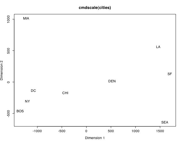
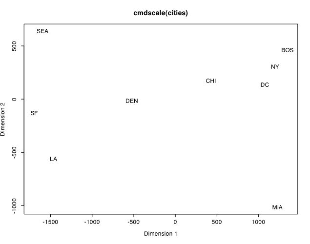
Note that the solution is not quite what we expected (it is giving us a mirrored Australian orientation to American cities.) However, by reversing the signs in city.location, we get the more conventional representation:

city.location <- -city.location
plot(city.location,type="n", xlab="Dimension 1", ylab="Dimension 2",main ="cmdscale(cities)")    #put up a graphics window
text(city.location,labels=names(cities))     #put the cities into the map

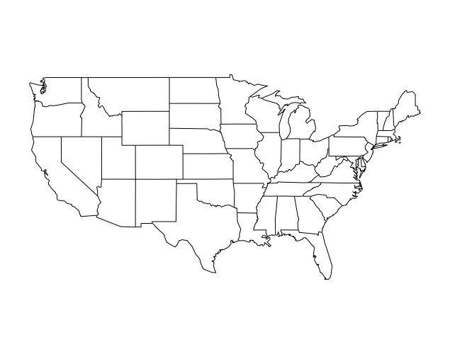
(Using the maps package we can compare this solution to a map of the US.

map("state")

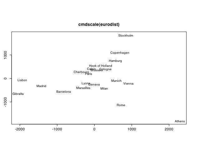
A useful feature is R is most commands have an extensive help file. Asking for help(cmdscale) shows that R includes a distance matrix for 20 European cities. The following commands (taken from the help file) produce a nice two dimensional solution. (Note that since dimensions are arbitrary, the second dimension needs to be flipped to produce the conventional map of Europe.)

loc <- cmdscale(eurodist)
x <- loc[,1]
y <- -loc[,2]
plot(x, y, type="n", xlab="", ylab="", main="cmdscale(eurodist)")
text(x, y, names(eurodist), cex=0.8)