Determining the optimal number of interpretable factors by using Very Simple Structure
The classic factor model is that elements of a correlation matrix (R) may be approximated by the product of a factor matrix (F) times the transpose of F (F') plus a diagonal matrix of uniquenesses U²:
nRn ~ nFkkF'n + nU²n.
Determining the appropriate number of factors from a factor analysis is perhaps one of the greatest challenges in factor analysis. There are many solutions to this problem, none of which is uniformly the best. "Solving the number of factors problem is easy, I do it everyday before breakfast. But knowing the right solution is harder" (Kaiser, 195x).
Techniques most commonly used include
- Chi Square rule #1: Extracting factors until the chi square of the residual matrix is not significant.
- Chi Square rule #2: Extracting factors until the change in chi square from factor n to factor n+1 is not significant.
- Parallel Analysis: Extracting factors until the eigen values of the real data are less than the corresponding eigen values of a random data set of the same size.
- Scree Test: Plotting the magnitude of the successive eigen values and applying the scree test (a sudden drop in eigen values analogous to the change in slope seen when scrambling up the talus slope of a mountain and approaching the rock face).
- Eigen Value of 1 rule: Extracting principal components until the eigen value <1.
- Meaning: Extracting factors as long as they are interpetable.
- VSS: Using the Very Simple Structure Criterion.
Each of the procedures has its advantages and disadvantages. Using either the chi square test or the change in square test is, of course, sensitive to the number of subjects and leads to the nonsensical condition that if one wants to find many factors, one simply runs more subjects. Parallel analysis is partially sensitive to sample size in that for large samples the eigen values of random factors will be very small. The scree test is quite appealling but can lead to differences of interpretation as to when the scree "breaks". The eigen value of 1 rule, although the default for many programs, seems to be a rough way of dividing the number of variables by 3. Extracting interpretable factors means that the number of factors reflects the investigators creativity more than the data. VSS, while very simple to understand, will not work very well if the data are very factorially complex. (Simulations suggests it will work fine if the complexities of some of the items are no more than 2).
Most users of factor analysis tend to interpret factor output by focusing their attention on the largest loadings for every variable and ignoring the smaller ones. Very Simple Structure operationalizes this tendency by comparing the original correlation matrix to that reproduced by a simplified version (S) of the original factor matrix (F). R ~ SS' + U². S is composed of just the c greatest (in absolute value) loadings for each variable. C (or complexity) is a parameter of the model and may vary from 1 to the number of factors.
The VSS criterion compares the fit of the simplified model to the original correlations: VSS = 1 -sumsquares(r*)/sumsquares(r) where R* is the residual matrix R* = R - SS' and r* and r are the elements of R* and R respectively.
VSS for a given complexity will tend to peak at the optimal (most interpretable) number of factors (Revelle and Rocklin, 1979).
Although originally written in Fortran for main frame computers, VSS has been adapted to micro computers (e.g., Macintosh OS 6-9) using Pascal. With the availability of an extremely powerful public domain statistical package R, we now release R code for calculating VSS. This is a preliminary release, with further modifications to make it a package within the R system. For an introduction in R for psychologists, see tutorials by Baron and Li or Revelle.
Installing VSS in R
To use this code within R, simply copy the following command into R to load VSS and associated functions:
source("http://personality-project.org/r/vss.r")
Using VSS
In R, for a data matrix "my.data" issue the call:my.vss <- VSS(mydata,n=8,rotate="none",diagonal=FALSE,...) #compares up to 8 factors VSS.plot(my.vss)
To compare the VSS result to a scree test, find the correlation matrix and then call VSS.scree which finds and plots the eigen values of the principal components of the correlation matrix.
VSS.scree(cor(mydata), main ="scree plot")
Output from VSS is a data.frame with n (number of factors to try) rows and 21 elements:
"dof" degrees of freedom in the model for this number of factors
"chisq" chi square for the the model
"prob" probability of chi square
"sqresid" the sum of the squared residuals for the full (non simple) model
"fit" fit statistic for full model
"cfit.1" fit statistic for complexity 1 (VSS 1)
"cfit.2" fit statistic for complexity 2
"cfit.3" ...
"cfit.4"
"cfit.5"
"cfit.6"
"cfit.7"
"cfit.8"
"cresidual.1" sum squares of residual correlations for complexity 1
"cresidual.2"
"cresidual.3"
"cresidual.4"
"cresidual.5"
"cresidual.6"
"cresidual.7"
"cresidual.8"
This output does not need to be displayed, but can rather be plotted using VSS.plot.
Additional functions that are part of a VSS package include functions to do parallel analyses and generate a simple structure for a particular number of factors and variables.
Very Simple Structure
The first figure compares the fit with or without the main diagonal as a function of the number of factors in the data.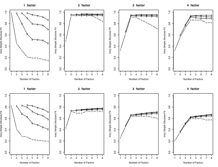
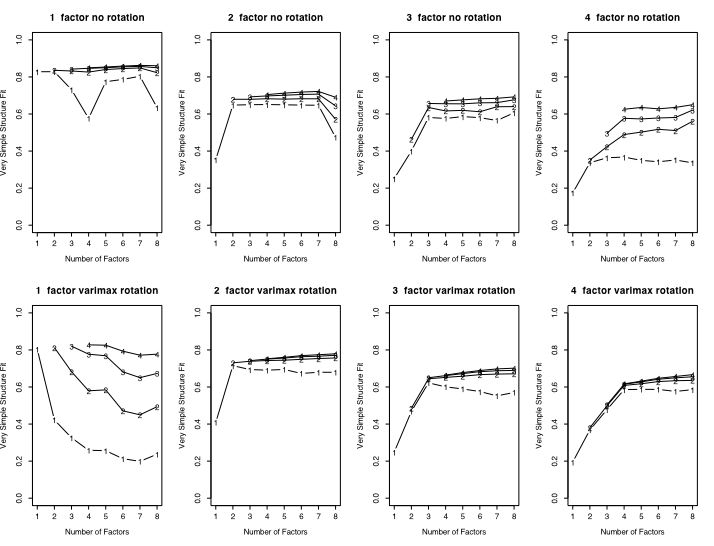
VSS with and without rotations
The second figure shows the fit as function of number of simulated factors and whether varimax or no rotation was done.
Code listing and examples
The following code is a more extensively annotated version of what is loaded, along with some examples.
#Very Simple Structure     (version of November 7, 2004: revised May 15, 2005)
#William Revelle
#Department of Psychology, Northwestern University
#revelle @ northwestern.edu
#a method for determining the most interpretable number of factors to extract
#written as a function library  to allow for easier use (eventually)
#
#see Revelle and Rocklin, 1979 for basic algorithm and justification of program
#see http://personality-project.org/r/vss.html for more detail
#makes repeated calls to the factor analysis package (factanal) of R
#parameter calls to VSS are similar to those of factanal

#things to do: add feature allowing for VSS applied to principal components
#add feature to allow doing VSS on specified correlation and factor matrices
#VSS=function (x,n=8,rotate="none",diagonal=FALSE,...)     #apply the Very Simple Structure Criterion for up to n factors on data set x
#VSS.plot<- function(x,plottitle="Very Simple Structure",line=FALSE)
#VSS.simulate <-function(ncases,nvariables,nfactors,meanloading)     #generates a simple structure factor matrix

VSS=function (x,n=8,rotate="none",diagonal=FALSE,...)     #apply the Very Simple Structure Criterion for up to n factors on data set x
  #x is a data matrix
  #n is the maximum number of factors to extract  (default is 8)
  #rotate is a string "none" or "varimax" for type of rotation (default is "none"
  #diagonal is a boolean value for whether or not we should count the diagonal  (default=FALSE)
  # ... other parameters for factanal may be passed as well
  #e.g., to do VSS on a covariance/correlation matrix with up to 8 factors and 3000 cases:
  #VSS(covmat=msqcovar,n=8,rotate="none",n.obs=3000)


 {             #start Function definition
  #first some preliminary functions

  #complexrow sweeps out all except the c largest loadings
  #complexmat applies complexrow to the loading matrix


complexrow <- function(x,c)     #sweep out all except c loadings
    {  n=length(x)          	#how many columns in this row?
       temp <- x                #make a temporary copy of the row
       x <- rep(0,n)            #zero out x
       for (j in 1:c)
       {
       	locmax <- which.max(abs(temp))                     #where is the maximum (absolute) value
      	 x[locmax] <- sign(temp[locmax])*max(abs(temp))    #store it in x
       	temp[locmax] <- 0                                  #remove this value from the temp copy
       }
     return(x)                                             #return the simplified (of complexity c) row
    }

 complexmat <- function(x,c)           #do it for every row   (could tapply somehow?)
	{
	nrows <- dim(x)[1]
	ncols <- dim(x)[2]
	for (i in 1:nrows)
   		{x[i,] <- complexrow(x[i,],c)}   #simplify each row of the loading matrix
 	return(x)
	 }

  #now do the main Very Simple Structure  routine

  complexfit <- array(0,dim=c(n,n))        #store these separately for complex fits
  complexresid <-  array(0,dim=c(n,n))

  vss.df <- data.frame(dof=rep(0,n),chisq=0,prob=0,sqresid=0,fit=0) #keep the basic results here
 for (i in 1:n)                            #loop through 1 to the number of factors requested
 {
   f <- factanal(x,i,rotation=rotate,...)  #do a factor analysis with i factors and the rotations specified in the VSS call
 	 if (i==1)
  		 {original <- f$correlation         #just find this stuff once
		 sqoriginal <- original*original    #squared correlations
		 totaloriginal <- sum(sqoriginal) - diagonal*sum(diag(sqoriginal) )   #sum of squared correlations - the diagonal
		}

 	load <- f$loadings                      #the loading matrix
  	model <- load%*%t(load)                 #reproduce the correlation matrix by the factor law R ≈ FF'
 	residual <- original-model              #find the residual  R* = R - FF'
 	sqresid <- residual*residual            #square the residuals
 	totalresid <- sum(sqresid)- diagonal * sum(diag(sqresid) )      #sum squared residuals - the main diagonal
 	fit <- 1-totalresid/totaloriginal       #fit is 1-sumsquared residuals/sumsquared original     (of off diagonal elements

 	vss.df[i,1] <- f$dof                   #degrees of freedom from the factor analysis
 	vss.df[i,2] <- f$STATISTIC             #chi square from the factor analysis
 	vss.df[i,3] <- f$PVAL                  #probability value of this complete solution
  	vss.df[i,4] <- totalresid              #residual given complete model
  	vss.df[i,5] <- fit                     #fit of complete model


     #now  do complexities -- how many factors account for each item

  for (c in 1:i)

  	 {
  	 	simpleload <- complexmat(load,c)             #find the simple structure version of the loadings for complexity c
  		model <- simpleload%*%t(simpleload)           #the model is now a simple structure version  R ≈ SS'
  		residual <- original- model                   #R* = R - SS'
  		sqresid <- residual*residual
  		totalsimple <- sum(sqresid) -diagonal * sum(diag(sqresid))    #default is to not count the diagonal
  		simplefit <- 1-totalsimple/totaloriginal
  		complexresid[i,c] <-totalsimple
  		complexfit[i,c] <- simplefit
  	 }

}     #end of i loop for number of factors


vss.stats <- data.frame(vss.df,cfit=complexfit,cresidual=complexresid)
return(vss.stats)

    }     #end of VSS function

#####################################################################
#function to plot the output of VSS
#Only plots complexities 1-4
#


VSS.plot<- function(x,plottitle="Very Simple Structure",line=FALSE)
  {
  	n=dim(x)
  	symb=c(49,50,51,52)              #plotting sym
	plot(x$cfit.1,ylim=c(0,1),type="b",ylab="Very Simple Structure Fit",xlab="Number of Factors",pch=49)
    if (line) lines(x$fit)


	title(main=plottitle)
	x$cfit.2[1]<-NA
	x$cfit.3[1]<-NA
	x$cfit.3[2]<-NA
	x$cfit.4[1]<-NA
	x$cfit.4[2]<-NA
	x$cfit.4[3]<-NA
	lines(x$cfit.2)
	points(x$cfit.2,pch=50)
	lines(x$cfit.3)
	points(x$cfit.3,pch=symb[3])
	lines(x$cfit.4)
	points(x$cfit.4,pch=symb[4])
}


#######
#generates random data to do parallel analyses to check VSS against random data

VSS.parallel <- function(ncases,nvariables)       #function call
{
 simdata=matrix(rnorm(ncases*nvariables),nrow=ncases,ncol=nvariables)    #make up simulated data
 testsim <- VSS(simdata,8,"none")
 return(testsim)
 }


######################################################################################

VSS.simulate <-function(ncases,nvariables,nfactors,meanloading)     #generates a simple structure factor matrix
                                                                    #with nfactors

{
weight=sqrt(1-meanloading*meanloading)                            #loadings are path coefficients
theta=matrix(rnorm(ncases*nfactors),nrow=ncases,ncol=nvariables)  #generates nfactor independent columns, repeated nvariable/nfactor times)
error=matrix(rnorm(ncases*nvariables),nrow=ncases,ncol=nvariables) #errors for all variables
items=meanloading*theta+weight*error                               #observed score = factor score + error score
return(items)
}

#####################################################
Output from VSS is a data.frame with n (number of factors to try) rows and 21 elements:
"dof" degrees of freedom in the model for this number of factors
"chisq" chi square for the the model
"prob" probability of chi square
"sqresid" the sum of the squared residuals for the full (non simple) model
"fit" fit statistic for full model
"cfit.1" fit statistic for complexity 1 (VSS 1)
"cfit.2" fit statistic for complexity 2
"cfit.3" ...
"cfit.4"
"cfit.5"
"cfit.6"
"cfit.7"
"cfit.8"
"cresidual.1" sum squares of residual correlations for complexity 1
"cresidual.2"
"cresidual.3"
"cresidual.4"
"cresidual.5"
"cresidual.6"
"cresidual.7"
"cresidual.8"
This output does not need to be displayed, but can rather be plotted using plotVSS.
Additional functions that are part of a VSS package include functions to do parallel analyses and generate a simple structure for a particular number of factors and variables.
#######
#generates random data to do parallel analyses to check VSS against random data

VSS.parallel <- function(ncases,nvariables)       #function call
{
 simdata=matrix(rnorm(ncases*nvariables),nrow=ncases,ncol=nvariables)    #make up simulated data
 testsim <- VSS(simdata,8,"none")
 return(testsim)
 }


######################################################################################

VSS.simulate <-function(ncases,nvariables,nfactors,meanloading)     #generates a simple structure factor matrix
                                                                    #with nfactors

{
weight=sqrt(1-meanloading*meanloading)                            #loadings are path coefficients
theta=matrix(rnorm(ncases*nfactors),nrow=ncases,ncol=nvariables)  #generates nfactor independent columns, repeated nvariable/nfactor times)
error=matrix(rnorm(ncases*nvariables),nrow=ncases,ncol=nvariables) #errors for all variables
items=meanloading*theta+weight*error                               #observed score = factor score + error score
return(items)
}
Demonstrations of these functions and the graphics they produce are
# test out VSS with 1 - 4 factors
meanloading <- .5               #this implies item * item intercorrelations of .25 within a factor, actually fairly typical
ncases <- 400                   #typical sample size
nvar <- 36                   #typical problem size

par(mfrow=c(2,4))            #2 rows and 4 columns allow us to compare results

#this first set removes the diagonal values and fits the off diagonal elements

for (i in 1:4)
{ x=VSS(VSS.simulate(ncases,nvar,i,meanloading),diagonal=TRUE,rotate="varimax")
VSS.plot(x,paste(i, " factor"),line=FALSE) }


#this set leaves the diagonal on and thus fits are worse

for (i in 1:4)
{ x <- VSS(VSS.simulate(ncases,36,i,meanloading),rotate="varimax")
VSS.plot(x,paste(i, " factor"),line=FALSE) }


#these next 8 analyses compare varimax to no rotations
#it seems as if VSS better detects the number of factors with rotated solutions
par(mfrow=c(2,4))            #2 rows and 4 columns allow us to compare results

for (i in 1:4)
{ x=VSS(VSS.simulate(ncases,nvar,i,meanloading),rotate="none")
VSS.plot(x,paste(i, " factor no rotation"),line=FALSE) }

for (i in 1:4)
{ x=VSS(VSS.simulate(ncases,nvar,i,meanloading),rotate="varimax")
VSS.plot(x,paste(i, " factor varimax rotation"),line=FALSE) }
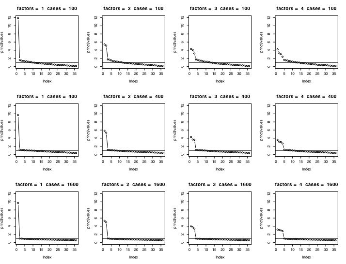
The scree test
The next figure compares the scree test and the eigen value of 1 rule for 1 .. 4 factors for sample sizes of small (100), medium (400) and large (1600) numbers of subjects.
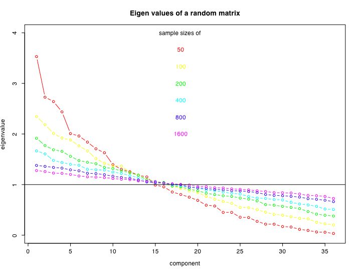
Parallel Analysis
The final figure compares the size of the eigen values for random data matrices of size 36 for sample sizes ranging from 50 to 1600.
Two factor circumplex data without and with skew
The next set of figures compares VSS and the scree test for a two dimensional data set with and without skewed items. Skew was introduced by truncating all responses below 0 to be 0. (See Rafaeli and Revelle, 2005 for a discussion of the problem in skew in measuring mood.)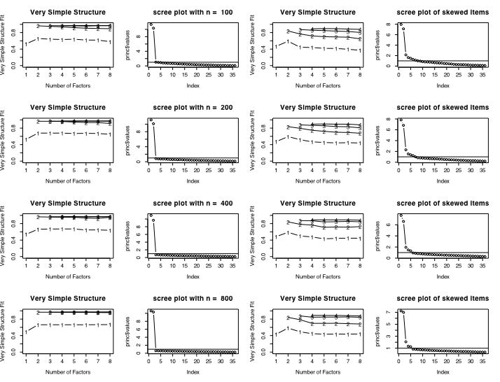
part of a short guide to R
Version of May 15, 2005
William Revelle
Department of Psychology
Northwestern University