Revelle (1979) proposed that hierachical cluster analysis could be used to estimate a new coefficient (beta) that was an estimate of the general factor saturation of a test. More recently, Zinbarg, Revelle, Yovel and Li (2005) compared McDonald's Omega to Chronbach's alpha and Revelle's beta. They conclude that omega is the best estimate. An algorithm for estimating omega using R is available as part of the "psych" package at http://personality-project.org/r.
Although ICLUST was originally written in FORTRAN for a CDC 6400 and then converted for IBM mainframes, Cooksey and Soutar, (2005) report using a PC adaptation of the original FORTRAN program. A modified version, written in Lightspeed Pascal has been available for the Mac for several years but did not have all the graphic features of the original program.
I now release a completely new version of ICLUST, written in R. It is still under development but is included as part of the "psych" package. Although early testing suggests it is stable, let me know if you have problems. Please email me if you want help with this version of ICLUST or if you desire more features.
The program currently has three primary functions: cluster, loadings, and graphics. There is no documentation yet for the program, although one can figure out most requirements by reading the code.
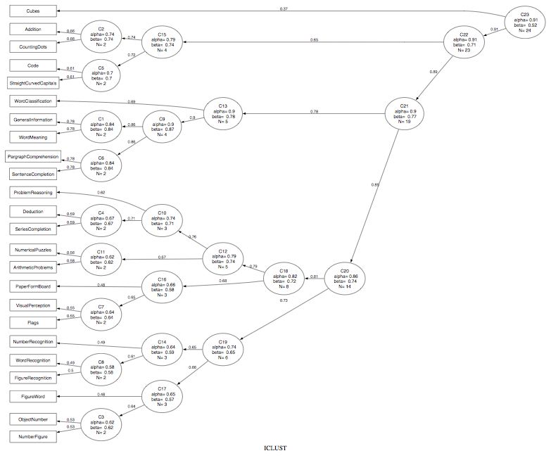
A sample output using the 24 variable problem by Harman can be represented both graphically and in terms of the cluster order. Note that the graphic is created using GraphViz in the dot language. ICLUST.graph produces the dot code for Graphviz. I have also tried doing this in Rgraphviz with less than wonderful results. Dot code can be viewed directly in Graphviz or can be tweaked using commercial software packages (e.g., OmniGraffle)
Note that for this problem, with these parameters, the data formed one large cluster. (This is consistent with the Very Simple Structure (VSS) output as well, which shows a clear one factor solution for complexity 1 data.) See below for an example with this same data set, but with more stringent parameter settings.
 r.mat<- Harman74.cor$cov
 iq.clus <- ICLUST(r.mat)
 ICLUST.graph(iq.clus,title="ICLUST of 24 mental variables",out.file="iclust.dot")


$title
[1] "ICLUST"

$clusters
      VisualPerception                  Cubes         PaperFormBoard                  Flags     GeneralInformation  PargraphComprehension
                     1                      1                      1                      1                      1                      1
    SentenceCompletion     WordClassification            WordMeaning               Addition                   Code           CountingDots
                     1                      1                      1                      1                      1                      1
StraightCurvedCapitals        WordRecognition      NumberRecognition      FigureRecognition           ObjectNumber           NumberFigure
                     1                      1                      1                      1                      1                      1
            FigureWord              Deduction       NumericalPuzzles       ProblemReasoning       SeriesCompletion     ArithmeticProblems
                     1                      1                      1                      1                      1                      1

$corrected
     [,1]
[1,]    1

$loadings
                       [,1]
VisualPerception       0.55
Cubes                  0.34
PaperFormBoard         0.38
Flags                  0.44
GeneralInformation     0.60
PargraphComprehension  0.59
SentenceCompletion     0.57
WordClassification     0.60
WordMeaning            0.59
Addition               0.41
Code                   0.51
CountingDots           0.43
StraightCurvedCapitals 0.55
WordRecognition        0.39
NumberRecognition      0.37
FigureRecognition      0.48
ObjectNumber           0.44
NumberFigure           0.49
FigureWord             0.42
Deduction              0.56
NumericalPuzzles       0.55
ProblemReasoning       0.56
SeriesCompletion       0.63
ArithmeticProblems     0.60

$fit
$fit$clusterfit
[1] 0.76

$fit$factorfit
[1] 0.76


$results
    Item/Cluster Item/Cluster similarity correlation alpha1 alpha2 beta1 beta2 size1 size2 rbar1 rbar2   r1   r2 alpha beta rbar size
C1            V9           V5       1.00        0.72   0.72   0.72  0.72  0.72     1     1  0.72  0.72 0.78 0.78  0.84 0.84 0.72    2
C2           V12          V10       1.00        0.58   0.58   0.58  0.58  0.58     1     1  0.58  0.58 0.66 0.66  0.74 0.74 0.58    2
C3           V18          V17       1.00        0.45   0.45   0.45  0.45  0.45     1     1  0.45  0.45 0.53 0.53  0.62 0.62 0.45    2
C4           V23          V20       1.00        0.51   0.51   0.51  0.51  0.51     1     1  0.51  0.51 0.59 0.59  0.67 0.67 0.51    2
C5           V13          V11       1.00        0.54   0.54   0.54  0.54  0.54     1     1  0.54  0.54 0.61 0.61  0.70 0.70 0.54    2
C6            V7           V6       1.00        0.72   0.72   0.72  0.72  0.72     1     1  0.72  0.72 0.78 0.78  0.84 0.84 0.72    2
C7            V4           V1       0.98        0.47   0.47   0.48  0.47  0.48     1     1  0.47  0.48 0.55 0.55  0.64 0.64 0.47    2
C8           V16          V14       0.98        0.41   0.43   0.41  0.43  0.41     1     1  0.43  0.41 0.50 0.49  0.58 0.58 0.41    2
C9            C1           C6       0.93        0.78   0.84   0.84  0.84  0.84     2     2  0.72  0.72 0.86 0.86  0.90 0.87 0.69    4
C10           C4          V22       0.91        0.56   0.67   0.56  0.67  0.56     2     1  0.51  0.56 0.71 0.62  0.74 0.71 0.49    3
C11          V21          V24       0.86        0.45   0.51   0.53  0.51  0.53     1     1  0.51  0.53 0.56 0.58  0.62 0.62 0.45    2
C12          C10          C11       0.86        0.58   0.74   0.62  0.71  0.62     3     2  0.49  0.45 0.76 0.67  0.79 0.74 0.43    5
C13           C9           V8       0.85        0.64   0.90   0.64  0.87  0.64     4     1  0.69  0.64 0.90 0.69  0.90 0.78 0.64    5
C14           C8          V15       0.84        0.41   0.58   0.41  0.58  0.41     2     1  0.41  0.41 0.61 0.49  0.64 0.59 0.37    3
C15           C2           C5       0.82        0.59   0.74   0.70  0.74  0.70     2     2  0.58  0.54 0.74 0.72  0.79 0.74 0.49    4
C16           V3           C7       0.81        0.41   0.41   0.64  0.41  0.64     1     2  0.41  0.47 0.48 0.65  0.66 0.58 0.39    3
C17          V19           C3       0.80        0.40   0.41   0.62  0.41  0.62     1     2  0.41  0.45 0.48 0.64  0.65 0.57 0.38    3
C18          C12          C16       0.78        0.57   0.79   0.66  0.74  0.58     5     3  0.43  0.39 0.79 0.68  0.82 0.72 0.37    8
C19          C17          C14       0.76        0.49   0.64   0.64  0.57  0.59     3     3  0.38  0.37 0.66 0.65  0.74 0.65 0.32    6
C20          C18          C19       0.76        0.59   0.82   0.74  0.72  0.65     8     6  0.37  0.32 0.81 0.73  0.86 0.74 0.30   14
C21          C20          C13       0.71        0.62   0.86   0.90  0.74  0.78    14     5  0.30  0.64 0.85 0.78  0.90 0.77 0.32   19
C22          C15          C21       0.65        0.55   0.79   0.90  0.74  0.77     4    19  0.49  0.32 0.65 0.89  0.91 0.71 0.31   23
C23          C22           V2       0.62        0.35   0.91   0.35  0.71  0.35    23     1  0.31  0.35 0.91 0.37  0.91 0.52 0.30   24

$cor
     [,1]
[1,]    1

$alpha
[1] 0.91

$size
[1] 24
Graphviz (or OmniGraffle) can open the dot file (ICLUST.dot) and will show the figure. (See above). The dot file can be edited with a normal text editor to make the figure cleaner.
The previous solution showed that all 24 mental tests formed one, high level cluster (g). An alternative is to form smaller, tighter clusters. These were formed, of course, in the previous analysis, but it would be nice to find the correlations, loadings, and fit statistics for a multiple cluster solution.
Note that the cluster fit, and the more stringent factor fit are worse for this solution than the previous solution. Also note that one of the "clusters" is a single variable (cubes).
r.mat<- Harman74.cor$cov
iq.clus <- ICLUST(r.mat,nclusters=4)
graph.out <- file.choose()
ICLUST.graph(iq.clus,graph.out,title = "ICLUST of 24 mental variables")
iq.clus

$title
[1] "ICLUST"

$clusters
                       V2 C13 C15 C20
VisualPerception        0   0   0   1
Cubes                   1   0   0   0
PaperFormBoard          0   0   0   1
Flags                   0   0   0   1
GeneralInformation      0   1   0   0
PargraphComprehension   0   1   0   0
SentenceCompletion      0   1   0   0
WordClassification      0   1   0   0
WordMeaning             0   1   0   0
Addition                0   0   1   0
Code                    0   0   1   0
CountingDots            0   0   1   0
StraightCurvedCapitals  0   0   1   0
WordRecognition         0   0   0   1
NumberRecognition       0   0   0   1
FigureRecognition       0   0   0   1
ObjectNumber            0   0   0   1
NumberFigure            0   0   0   1
FigureWord              0   0   0   1
Deduction               0   0   0   1
NumericalPuzzles        0   0   0   1
ProblemReasoning        0   0   0   1
SeriesCompletion        0   0   0   1
ArithmeticProblems      0   0   0   1

$corrected
      V2  C13  C15  C20
V2  1.00 0.26 0.21 0.41
C13 0.24 0.90 0.47 0.71
C15 0.19 0.40 0.79 0.67
C20 0.38 0.62 0.55 0.86

$loadings
                         V2  C13  C15  C20
VisualPerception       0.32 0.38 0.39 0.57
Cubes                  1.00 0.24 0.19 0.38
PaperFormBoard         0.32 0.31 0.15 0.42
Flags                  0.23 0.38 0.22 0.45
GeneralInformation     0.28 0.77 0.39 0.50
PargraphComprehension  0.23 0.77 0.31 0.53
SentenceCompletion     0.16 0.80 0.32 0.49
WordClassification     0.16 0.67 0.40 0.56
WordMeaning            0.20 0.79 0.27 0.54
Addition               0.06 0.29 0.63 0.35
Code                   0.15 0.36 0.61 0.48
CountingDots           0.14 0.21 0.65 0.40
StraightCurvedCapitals 0.24 0.40 0.62 0.51
WordRecognition        0.10 0.31 0.27 0.41
NumberRecognition      0.13 0.26 0.22 0.41
FigureRecognition      0.27 0.28 0.27 0.56
ObjectNumber           0.00 0.29 0.36 0.47
NumberFigure           0.26 0.25 0.43 0.54
FigureWord             0.11 0.29 0.27 0.46
Deduction              0.29 0.51 0.27 0.58
NumericalPuzzles       0.31 0.36 0.50 0.54
ProblemReasoning       0.23 0.49 0.30 0.58
SeriesCompletion       0.35 0.54 0.40 0.62
ArithmeticProblems     0.21 0.50 0.54 0.54

$fit
$fit$clusterfit
[1] 0.51

$fit$factorfit
[1] 0.16


$results
    Item/Cluster Item/Cluster similarity correlation alpha1 alpha2 beta1 beta2 size1 size2 rbar1 rbar2   r1   r2 alpha beta rbar size
C1            V9           V5       1.00        0.72   0.72   0.72  0.72  0.72     1     1  0.72  0.72 0.78 0.78  0.84 0.84 0.72    2
C2           V12          V10       1.00        0.58   0.58   0.58  0.58  0.58     1     1  0.58  0.58 0.66 0.66  0.74 0.74 0.58    2
C3           V18          V17       1.00        0.45   0.45   0.45  0.45  0.45     1     1  0.45  0.45 0.53 0.53  0.62 0.62 0.45    2
C4           V23          V20       1.00        0.51   0.51   0.51  0.51  0.51     1     1  0.51  0.51 0.59 0.59  0.67 0.67 0.51    2
C5           V13          V11       1.00        0.54   0.54   0.54  0.54  0.54     1     1  0.54  0.54 0.61 0.61  0.70 0.70 0.54    2
C6            V7           V6       1.00        0.72   0.72   0.72  0.72  0.72     1     1  0.72  0.72 0.78 0.78  0.84 0.84 0.72    2
C7            V4           V1       0.98        0.47   0.47   0.48  0.47  0.48     1     1  0.47  0.48 0.55 0.55  0.64 0.64 0.47    2
C8           V16          V14       0.98        0.41   0.43   0.41  0.43  0.41     1     1  0.43  0.41 0.50 0.49  0.58 0.58 0.41    2
C9            C1           C6       0.93        0.78   0.84   0.84  0.84  0.84     2     2  0.72  0.72 0.86 0.86  0.90 0.87 0.69    4
C10           C4          V22       0.91        0.56   0.67   0.56  0.67  0.56     2     1  0.51  0.56 0.71 0.62  0.74 0.71 0.49    3
C11          V21          V24       0.86        0.45   0.51   0.53  0.51  0.53     1     1  0.51  0.53 0.56 0.58  0.62 0.62 0.45    2
C12          C10          C11       0.86        0.58   0.74   0.62  0.71  0.62     3     2  0.49  0.45 0.76 0.67  0.79 0.74 0.43    5
C13           C9           V8       0.85        0.64   0.90   0.64  0.87  0.64     4     1  0.69  0.64 0.90 0.69  0.90 0.78 0.64    5
C14           C8          V15       0.84        0.41   0.58   0.41  0.58  0.41     2     1  0.41  0.41 0.61 0.49  0.64 0.59 0.37    3
C15           C2           C5       0.82        0.59   0.74   0.70  0.74  0.70     2     2  0.58  0.54 0.74 0.72  0.79 0.74 0.49    4
C16           V3           C7       0.81        0.41   0.41   0.64  0.41  0.64     1     2  0.41  0.47 0.48 0.65  0.66 0.58 0.39    3
C17          V19           C3       0.80        0.40   0.41   0.62  0.41  0.62     1     2  0.41  0.45 0.48 0.64  0.65 0.57 0.38    3
C18          C12          C16       0.78        0.57   0.79   0.66  0.74  0.58     5     3  0.43  0.39 0.79 0.68  0.82 0.72 0.37    8
C19          C17          C14       0.76        0.49   0.64   0.64  0.57  0.59     3     3  0.38  0.37 0.66 0.65  0.74 0.65 0.32    6
C20          C18          C19       0.76        0.59   0.82   0.74  0.72  0.65     8     6  0.37  0.32 0.81 0.73  0.86 0.74 0.30   14
C21            0            0       0.00        0.00   0.00   0.00  0.00  0.00     0     0  0.00  0.00 0.00 0.00  0.00 0.00 0.00    0
C22            0            0       0.00        0.00   0.00   0.00  0.00  0.00     0     0  0.00  0.00 0.00 0.00  0.00 0.00 0.00    0
C23            0            0       0.00        0.00   0.00   0.00  0.00  0.00     0     0  0.00  0.00 0.00 0.00  0.00 0.00 0.00    0

$cor
      V2  C13  C15  C20
V2  1.00 0.24 0.19 0.38
C13 0.24 1.00 0.40 0.62
C15 0.19 0.40 1.00 0.55
C20 0.38 0.62 0.55 1.00

$alpha
  V2  C13  C15  C20
1.00 0.90 0.79 0.86

$size
 V2 C13 C15 C20
  1   5   4  14
#ICLUST  - a function to form homogeneous item composites
# based upon Revelle, W. (1979). Hierarchical cluster analysis and the internal structure of tests. Multivariate Behavioral Research, 14, 57-74.
#
# psudo code
#	find similarity matrix
#		original is either covariance or correlation
#		corrected is disattenuated
#find most similar pair
#if size of pair > min size, apply beta criterion
#	if beta new > min(beta 1, beta 2) combine pair
#update similarity matrix
#repeat until finished
#then report various summary statistics
#example code
#r.mat<- Harman74.cor$cov
# print(ICLUST(r.mat),digits=2)

#ICLUST is the main function and calls other routines

"ICLUST" <-
 function (r.mat,nclusters=1,alpha=3,beta=1,beta.size=4,alpha.size=3,correct=TRUE,reverse=TRUE,beta.min=.5,output=1,digits=2,labels=NULL,cut=0,n.iterations=0,title="ICLUST") {#should allow for raw data, correlation or covariances
 #ICLUST.options <- list(n.clus=1,alpha=3,beta=2,beta.size=4,alpha.size=3,correct=TRUE,reverse=TRUE,beta.min=.5,output=1,digits=2)
	ICLUST.options <- list(n.clus=nclusters,alpha=alpha,beta=beta,beta.size=beta.size,alpha.size=alpha.size,correct=correct,reverse=reverse,beta.min=beta.min,output=output,digits=digits)
	if(dim(r.mat)[1]!=dim(r.mat)[2]) {r.mat <- cor(r.mat,use="pairwise") }    #cluster correlation matrices, find correlations if not square matrix
	iclust.results <- ICLUST.cluster(r.mat,ICLUST.options)
	loading <- cluster.loadings(iclust.results$clusters,r.mat,digits=digits)
	fits <- cluster.fit(r.mat,loading$loadings,iclust.results$clusters,digits=digits)
	sorted <- ICLUST.sort(ic.load=loading$loadings,labels=labels,cut=cut) #sort the loadings

	#now, iterate the cluster solution to clean it up (if desired)

		clusters <- iclust.results$clusters
		old.clusters <- clusters
		old.fit <- fits$clusterfit
		clusters <- factor2cluster(loading$loadings,cut=cut,loading=FALSE)
		load <- cluster.loadings(clusters,r.mat,digits=digits)
		if (n.iterations > 0) {  #it is possible to iterate the solution to perhaps improve it
		for (steps in 1:n.iterations) {   #
			load <- cluster.loadings(clusters,r.mat,digits=digits)
			clusters <- factor2cluster(loading$loadings,cut=cut,loading=FALSE)
			if(dim(clusters)[2]!=dim(old.clusters)[2]) {change <- 999
			load <- cluster.loadings(clusters,r.mat,digits=digits) } else {
			change <- sum(abs(clusters)-abs(old.clusters)) }  #how many items are changing?
			fit <- cluster.fit(r.mat,loading$loadings,clusters,digits=digits)
		old.clusters <- clusters
		print(paste("iterations ",steps," change in clusters ", change, "current fit " , fit$clusterfit))
		if ((abs(change) < 1) | (fit$clusterfit <= old.fit)) {break}    #stop iterating if it gets worse or there is no change in cluster definitions
		old.fit <- fit$cluster.fit
					}
		}
	p.fit <- cluster.fit(r.mat,loading$loadings,clusters,digits=digits)
	p.sorted <- ICLUST.sort(ic.load=loading$loadings,labels=labels,cut=cut)
	purified <- cluster.cor(clusters,r.mat,digits=digits)
	list(title=title,clusters=iclust.results$clusters,corrected=loading$corrected,loadings=loading$loadings,fit=fits,results=iclust.results$results,cor=loading$cor,alpha=loading$alpha,size=loading$size,sorted=sorted,p.fit = p.fit,p.sorted = p.sorted,purified=purified)
}

"ICLUST.sort"<- function (ic.load,cut=0,labels=NULL,loading=FALSE) {
     nclust <- dim(ic.load)[2]
     nitems <- dim(ic.load)[1]
    if (length(labels)==0) {
    var.labels <- rownames(ic.load)} else {var.labels=labels}
    if (length(var.labels)==0) {var.labels =paste('V',seq(1:nitems),sep='')} #unlabled variables
    if(loading) {loadings <- ic.load$loadings} else {loadings <- ic.load}


  loads <- data.frame(item=seq(1:nitems),content=var.labels,cluster=rep(0,nitems),loadings)

  #first find the maximum for each row and assign it to that cluster
   loads$cluster <- apply(abs(loadings),1,which.max)
  for (i in 1:nitems) {if (abs(loadings[i,loads$cluster[i]]) < cut) {loading$cluster[i] <- nclust+1}} #assign the ones that missed the cut a location

  ord <- sort(loads$cluster,index.return=TRUE)
  loads[1:nitems,] <- loads[ord$ix,]
  rownames(loads)[1:nitems] <- rownames(loads)[ord$ix]

  items <- c(table(loads$cluster),1)   #how many items are in each cluster?
  if(length(items) < (nclust+1)) {items <- rep(0,(nclust+1))   #this is a rare case where some clusters don't have anything in them
    for (i in 1:nclust+1) {items[i] <- sum(loads$cluster==i) }  }

  #now sort the loadings that have their highest loading on each cluster
   first <- 1
	for (i in 1:nclust) {
	if(items[i]>0 ) {
	last <- first + items[i]- 1
	ord <- sort(abs(loads[first:last,i+3]),decreasing=TRUE,index.return=TRUE)
   loads[first:last,] <- loads[ord$ix+first-1,]
    rownames(loads)[first:last] <- rownames(loads)[ord$ix+first-1]
    first <- first + items[i]}
    }
    if (first < nitems) loads[first:nitems,"cluster"] <- 0   #assign items less than cut to 0
 ICLUST.sort <- list(sorted=loads) }


ICLUST.cluster <- function (r.mat,ICLUST.options) {#should allow for raw data, correlation or covariances

#options:  alpha =1  (minimum alpha)  2 (average alpha)    3 (maximum alpha)
#          beta =1   (minimum beta)   2 (average beta)     3 (maximum beta)
#          correct  for reliability
#          reverse score items if negative correlations
#          stop clustering if beta for new clusters < beta.min
#          output =1 (short)    2  (show steps)     3 show rejects as we go

#initialize  various arrays and get ready for the first pass
output <- ICLUST.options$output
num.var <- nrow(r.mat)
keep.clustering <- TRUE          #used to determine when we are finished clustering
results <- data.frame(matrix(rep(0,18*(num.var-1)),ncol=18))
names(results) <- c("Item/Cluster", "Item/Cluster","similarity","correlation","alpha1","alpha2",
"beta1","beta2","size1","size2","rbar1","rbar2","r1","r2","alpha","beta","rbar","size")
rownames(results) <- paste("C",1:(num.var-1),sep="")

clusters <- diag(1,nrow =nrow(r.mat))    #original cluster structure is 1 item clusters
rownames(clusters) <- rownames(r.mat)
colnames(clusters) <- paste("V",1:num.var,sep="")
count=1

#master loop

while (keep.clustering) {   #loop until we figure out we should stop
#find similiarities
 #we will do most of the work on a copy of the r.mat
cluster.stats <- cluster.cor(clusters,r.mat,FALSE)
sim.mat <- cluster.stats$cor    #the correlation matrix
diag(sim.mat) <- 0   #we don't want 1's on the diagonal to mess up the maximum

#two ways to estimate reliability -- for 1 item clusters, max correlation, for >1, alpha
#this use of initial max should be an option
if (ICLUST.options$correct) {   #find the largest and smallest similarities for each variable
	row.range <- apply(sim.mat,1,range,na.rm=TRUE)
	row.max <- pmax(abs(row.range[1,]),abs(row.range[2,]))  #find the largest absolute similarity
   } else {row.max <- rep(1, nrow(sim)) }         #don't correct for largest similarity

   item.rel <-  cluster.stats$alpha
for (i in 1: length(item.rel)) { if (cluster.stats$size[i]<2) {
	item.rel[i] <- row.max[i]
	#figure out item betas here?
	}}
sq.max <- diag(1/sqrt(item.rel))     #used to correct for reliabilities
 #this is the corrected for maximum r similarities
if (ICLUST.options$correct) {sim <- sq.max %*% sim.mat %*% sq.max
     } else {sim <- sim.mat}
diag(sim) <- NA                  #we need to not consider the diagonal when looking for maxima
#find the most similar pair    and apply tests if we should combine
test.alpha <- FALSE
test.beta <- FALSE

while(!(test.alpha&test.beta)){

max.cell <- which.max(sim)             #global maximum
if (length(max.cell) < 1) {
   keep.clustering <- FALSE
   break}   #there are no non-NA values left
sign.max <- 1
if ( ICLUST.options$reverse ) {            #normal case is to reflect if necessary
	min.cell <- which.min(sim)             #location of global minimum
	if (sim[max.cell] <  abs(sim[min.cell] )) {
 	  	sign.max <- -1
		max.cell <- min.cell }
	if (sim[max.cell] < 0.0) {sign.max <- -1 }}
	               #this is a weird case where all the similarities are negative

max.col <- trunc(max.cell/nrow(sim))+1    #is in which row and column?
max.row <- max.cell - (max.col-1)*nrow(sim) #need to fix the case of first column
if (max.row < 1) {max.row <- nrow(sim)
 max.col <- max.col-1 }

#combine these two rows if the various criterion are passed
beta.combined <-  2* sign.max*sim.mat[max.cell]/(1+sign.max* sim.mat[max.cell])   #unweighted beta

size1 <- cluster.stats$size[max.row]
if(size1 < 2) {V1 <- 1
	beta1 <-  item.rel[max.row]
	alpha1 <-  item.rel[max.row]
	rbar1 <- item.rel[max.row] } else {
	rbar1 <- results[cluster.names[max.row],"rbar"]
	beta1 <- results[cluster.names[max.row],"beta"]
	alpha1 <- results[cluster.names[max.row],"alpha"]}

 V1 <- size1 + size1*(size1-1) * rbar1

size2 <- cluster.stats$size[max.col]
if(size2 < 2) {V2 <- 1
	beta2 <-  item.rel[max.col]
	alpha2 <-  item.rel[max.col]
	rbar2 <- item.rel[max.col] } else {
	rbar2 <- results[cluster.names[max.col],"rbar"]
	beta2 <- results[cluster.names[max.col],"beta"]
	alpha2 <- results[cluster.names[max.col],"alpha"]}

 V2 <- size2 + size2 * (size2-1) * rbar2

Cov12 <- sign.max* sim.mat[max.cell] * sqrt(V1*V2)
V12 <- V1 + V2 + 2 * Cov12
size12 <- size1 + size2
alpha <- (V12 - size12)*(size12/(size12-1))/V12
rbar <- alpha/(size12-alpha*(size12-1))

#what is the correlation of this new cluster with the two subclusters?
#this considers item overlap problems
c1 <-  sign.max*rbar1*size1*size1 + sign.max* Cov12   #corrects for item overlap
c2 <-  rbar2*size2*size2 + Cov12     #only flip one of the two correlations with the combined cluster
if(size1 > size2) {r1 <- c1/sqrt(V1*V12)
r2 <- sign.max* c2/sqrt(V2*V12) } else {r1 <-sign.max* c1/sqrt(V1*V12)
                                     #flip the smaller of the two clusters
r2 <-  c2/sqrt(V2*V12) }

#test if we should combine these two clusters
#first, does alpha increase?
test.alpha <- TRUE

if (ICLUST.options$alpha.size < min(size1,size2)) {
  switch(ICLUST.options$alpha, {if (alpha < min(alpha1,alpha2)) {if (output>2) {print(
  paste ('do not combine ', cluster.names[max.row],"with", cluster.names[max.col],
  'new alpha =', round (alpha,2),'old alpha1 =',round( alpha1,2),"old alpha2 =",round(alpha2,2)))}
												test.alpha <- FALSE }},
  {if (alpha < mean(alpha1,alpha2)) {if (output>2) {print(paste ('do not combine ',
  cluster.names[max.row],"with", cluster.names[max.col],'new alpha =', round (alpha,2),
  'old alpha1 =',round( alpha1,2),"old alpha2 =",round(alpha2,2)))}
												test.alpha <- FALSE  }},
  {if (alpha < max(alpha1,alpha2)) {if (output>2) {print(paste ('do not combine ',
  cluster.names[max.row],"with", cluster.names[max.col],'new alpha =', round (alpha,2),
  'old alpha1 =',round( alpha1,2),"old alpha2 =",round(alpha2,2)))}
												test.alpha <- FALSE  }}) #end switch
  }   #end if options$alpha.size

#second, does beta increase ?
test.beta <- TRUE

if (ICLUST.options$beta.size < min(size1,size2)) {
  switch(ICLUST.options$beta, {if (beta.combined < min(beta1,beta2)) {if (output>2) {print(
  paste ('do not combine ', cluster.names[max.row],"with", cluster.names[max.col],'new beta =',
  round (beta.combined,2),'old beta1 =',round( beta1,2),"old beta2 =",round(beta2,2)))}
												test.beta <- FALSE }},
  {if (beta.combined < mean(beta1,beta2)) {if (output>2) {print(paste ('do not combine ',
  cluster.names[max.row],"with", cluster.names[max.col],'new beta =', round (beta.combined,2),
  'old beta1 =',round( beta1,2),"old beta2 =",round(beta2,2)))}
												test.beta <- FALSE  }},
  {if (beta.combined < max(beta1,beta2)) {if (output>2) {print(paste ('do not combine ',
  cluster.names[max.row],"with", cluster.names[max.col],'new beta =', round (beta.combined,2),
  'old beta1 =',round( beta1,2),"old beta2 =",round(beta2,2)))}
												test.beta <- FALSE  }}) #end switch

  }   #end if options$beta.size


if(test.beta&test.alpha)   {break } else  {
if (beta.combined < ICLUST.options$beta.min) {
			keep.clustering <- FALSE       #the most similiar pair is not very similar, we should quit
			break}  else {sim[max.row,max.col] <- NA
		sim[max.col,max.row] <- NA }
    }   #end of test.beta&test.alpha

}    #end of while test.alpha&test.beta.loop

#combine and summarize
if (keep.clustering)
   {          # we have based the alpha and beta tests, now combine these two variables
clusters[,max.row] <- clusters[,max.row] + sign.max *  clusters[,max.col]
cluster.names <- colnames(clusters)

#summarize the results
results[count,1] <- cluster.names[max.row]
results[count,2] <- cluster.names[max.col]
results[count,"similarity"] <- sim[max.cell]
results[count,"correlation"] <- sim.mat[max.cell]
results[count,"alpha1"] <- item.rel[max.row]
results[count,"alpha2"] <- item.rel[max.col]
size1 <- cluster.stats$size[max.row]
size2 <- cluster.stats$size[max.col]
results[count,"size1"] <- size1
results[count,"size2"] <- size2
results[count,"beta1"] <-  beta1
results[count,"beta2"] <-  beta2
results[count,"rbar1"] <-  rbar1
results[count,"rbar2"] <-  rbar2
results[count,"r1"] <- r1
results[count,"r2"] <- r2


results[count,"beta"] <- beta.combined

results[count,'alpha'] <- alpha
results[count,'rbar'] <- rbar
results[count,"size"] <- size12
results[count,3:18] <- round(results[count,3:18],ICLUST.options$digits)
#update
cluster.names[max.row] <- paste("C",count,sep="")
colnames(clusters) <- cluster.names
clusters <- clusters[,-max.col]
cluster.names<- colnames(clusters)

#row.max <- row.max[-max.col]


	}  #end of combine section

if(output > 1) print(results[count,],digits=2)
count=count+1
if ((num.var - count) < ICLUST.options$n.clus) {keep.clustering <- FALSE}
if(num.var - count < 1) {keep.clustering <- FALSE}   #only one cluster left

}  #end of keep clustering loop

ICLUST.cluster <- list(results=results,clusters=clusters,number <- num.var - count)
}   # end ICLUST.cluster

cluster.loadings <-
function (keys, r.mat, correct = TRUE,digits=2)
{
    if (!is.matrix(keys))
        keys <- as.matrix(keys)
    item.covar <- r.mat %*% keys          #item by cluster covariances
    covar <- t(keys) %*% item.covar  #variance/covariance of clusters
    var <- diag(covar)
    sd.inv <- 1/sqrt(var)

    key.count <- diag(t(keys) %*% keys)    #how many items in each cluster?
    if (correct) {
                  cluster.correct <- diag((key.count/(key.count - 1)))
                   for (i in 1:ncol(keys)) {
                         if (key.count[i]==1) {   #fix the case of 1 item keys
                   	     cluster.correct[i,i] <- 1
                   	} else { cluster.correct[i,i] <- key.count[i]/(key.count[i]-1)
                   	item.covar[,i] <- item.covar[,i] - keys[,i]}
                   }   #i loop
                   correction.factor <- keys %*% cluster.correct
                   correction.factor[ correction.factor < 1] <- 1
                  item.covar <- item.covar * correction.factor
                  }


    ident.sd <- diag(sd.inv, ncol = length(sd.inv))
    cluster.loading <-  item.covar %*% ident.sd
    cluster.correl <- ident.sd %*% covar %*% ident.sd


    key.alpha <- ((var - key.count)/var) * (key.count/(key.count - 1))
    key.alpha[is.nan(key.alpha)] <- 1
    key.alpha[!is.finite(key.alpha)] <- 1
    colnames(cluster.loading) <- colnames(keys)
    colnames(cluster.correl) <- colnames(keys)
    rownames(cluster.correl) <- colnames(keys)
    rownames(cluster.loading) <- rownames(r.mat)

    if( ncol(keys) >1)  {cluster.corrected <- correct.cor(cluster.correl, t(key.alpha))} else {cluster.corrected <- cluster.correl}

    return(list(loadings=round(cluster.loading,digits), cor=round(cluster.correl,digits),corrected=round(cluster.corrected,digits), sd = round(sqrt(var),digits), alpha = round(key.alpha,digits),
            size = key.count))
    }


cluster.fit <- function(original,load,clusters,diagonal=FALSE,digits=2) {


 sqoriginal <- original*original    #squared correlations
 totaloriginal <- sum(sqoriginal) - diagonal*sum(diag(sqoriginal) )   #sum of squared correlations - the diagonal
        load <- as.matrix(load)
        clusters <- as.matrix(clusters)
        model <- load %*% t(load)                 #reproduce the correlation matrix by the factor law R=  FF'
        residual <- original-model              #find the residual  R* = R - FF'
        sqresid <- residual*residual            #square the residuals
        totalresid <- sum(sqresid)- diagonal * sum(diag(sqresid) )      #sum squared residuals - the main diagonal
        fit <- 1-totalresid/totaloriginal       #fit is 1-sumsquared residuals/sumsquared original     (of off diagonal elements
        clusters <- abs(clusters)
       model.1 <- (load * clusters) %*%  t(load*clusters)
       residual <- original - model.1
       sqresid <- residual*residual            #square the residuals
        totalresid <- sum(sqresid)- diagonal * sum(diag(sqresid) )      #sum squared residuals - the main diagonal
        fit.1 <- 1-totalresid/totaloriginal       #fit is 1-sumsquared residuals/sumsquared original     (of off diagonal elements
 cluster.fit <- list(clusterfit=round(fit.1,digits),factorfit=round(fit,digits))
 }