Adding time to a plot and adventures in smoothing
The following plots and instructions show how to put several figures on a page, give an overall label to the page, and to make time the axis. I also show how to subset the data to reject outliers. Finally, the effect of four levels of smoothing in 'lowess' are examined.
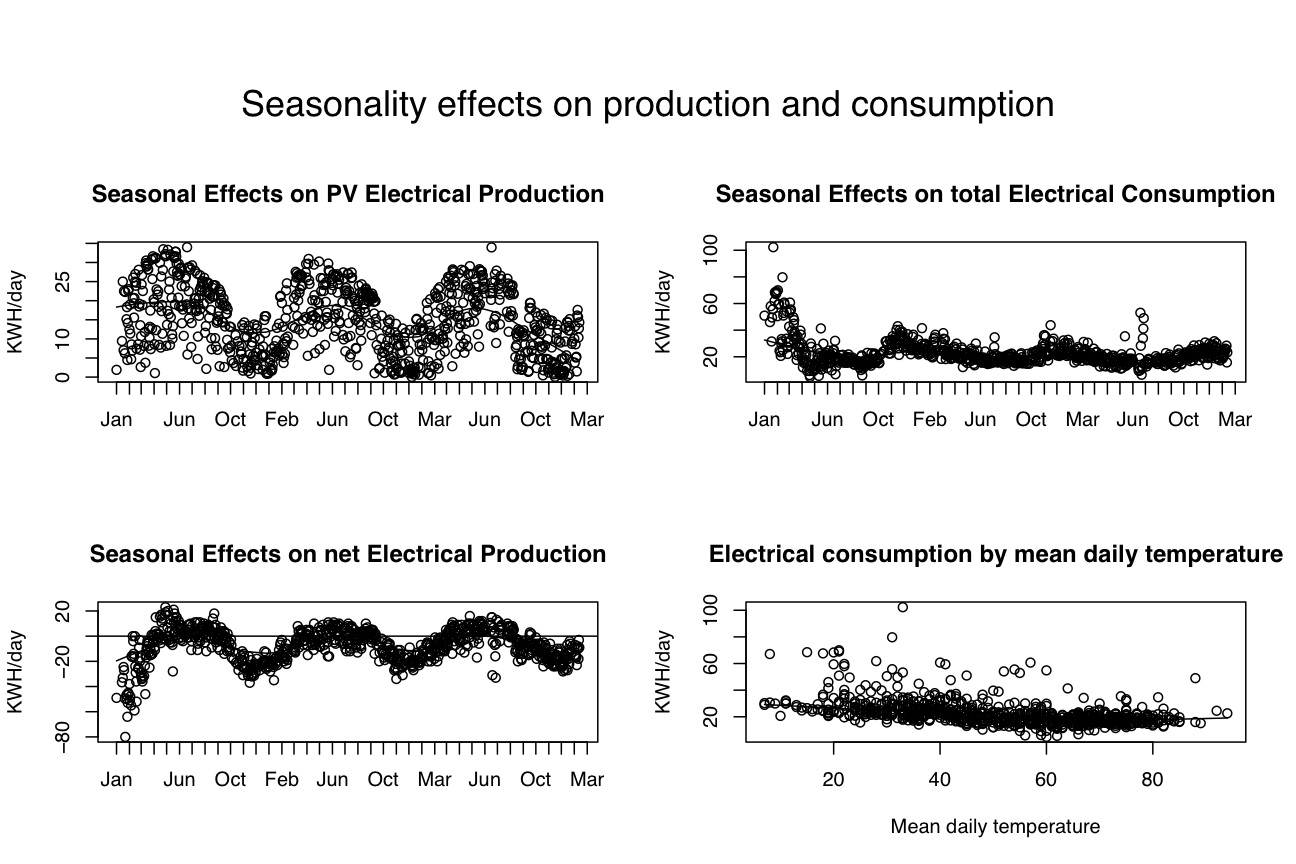
In order to show events over time, it is helpful to plot the data as a function of time. This is trivial if the data are equally spaced, but when the data are not equally spaced, it is important to add time to the plot. The following is an analysis of electrical production and consumption as a function of time of year for an energy efficient house. The data are from 38 months of fairly frequent observations of energy produced using PhotoVoltaic roofing and of electrical consumption.
The data are stored in a tab delimited text file produced by a spreadsheet. (e.g., Excel or Open Office)
datafilename="http://personality-project.org/r/datasets/electric.data.txt" #where are the data?
#local data are at datafilename <- "/Library/WebServer/Documents/personalitytheoryf/r/datasets/electric.data.txt"
#alternatively, we can dynamically find out the file name
datafilename <- file.choose()    #get the name of the file by using system commands

electric  <- read.table(datafilename,header=TRUE)  #read the data file
describe(electric)    #get basic descriptive statistics using the describe function

attach(electric)                               #for easier manipulation

dates <-strptime(as.character(electric$date1), "%m/%d/%y")   #change the date field to a internal form for time
                                                  #see ?formats and ?POSIXlt  for how to read different formats
                                                  #further note that we need to treat the date information as read from the spreadsheet as character data


electric=electric[,2:17]               #get rid of the original date in the data.frame
electric=data.frame(date=dates,electric)      #this is now the date in useful fashion

detach(electric)
daterange=c(as.POSIXlt(min(electric$date)),as.POSIXlt(max(electric$date)))   #figure out the lowest and highest months
rm(dates)       #get rid of the old date because otherwise it will be floating around confusing us
attach(electric)
#plot 4 different panels -- energy produced, consumed, net as function of date, concumption by temperature
quartz (height=6,width=9)      #create a graphic device of appropriate size
plot.new()                               #start a new plot
                                        #set parameters for this graph
par(omi=c(0,0,1,0) )                      #set the size of the outer margins
par(mfrow=c(2,2))                        #number of rows and columns to graph

plot(date,produced,xaxt="n",ylab="KWH/day")          #don't plot the x axis
axis.POSIXct(1, at=seq(daterange[1], daterange[2], by="month"), format="%b") #label the x axis by months
lines(lowess(date,produced, f=3/10))   #lowess smooth with 30% window
title(main="Seasonal Effects on PV Electrical Production")

plot(date,consumed,xaxt="n",ylab="KWH/day")          #don't plot the x axis
axis.POSIXct(1, at=seq(daterange[1], daterange[2], by="month"), format="%b") #label the x axis by months
lines(lowess(date,consumed, f=3/10))   #lowess smooth with 30% window
title(main="Seasonal Effects on total Electrical Consumption")

net=produced-consumed     #net electrical production
plot(date,net,xaxt="n",ylab="KWH/day")          #don't plot the x axis
axis.POSIXct(1, at=seq(daterange[1], daterange[2], by="month"), format="%b") #label the x axis by months
lines(lowess(date,net, f=3/10))   #lowess smooth with 30% window
title(main="Seasonal Effects on net Electrical Production")
abline(h=0)     #put in the net 0 line for readability

plot(temp1,consumed,main="Electrical consumption by mean daily temperature",xlab="Mean daily temperature",ylab="KWH/day")
#lines(lowess(mean,consumed,f=3/10))   #this does not work if there are missing data

#so, the following function fixes it
  lowess.na <- function(x, y = NULL, f = 2/3,...) {  #do lowess with missing data

  x1 <- subset(x,(!is.na(x)) &(!is.na(y)))
  y1 <- subset(y, (!is.na(x)) &(!is.na(y)))
  lowess.na <- lowess(x1,y1,f, ...)
  }

  lines(lowess.na(temp1,consumed,f=3/10))   #this does work if there are missing data


mtext("Seasonality effects on production and consumption",3,outer=TRUE,line=1,cex=1.5)    #note that we seem to add the global title last
                     #cex = character expansion factor
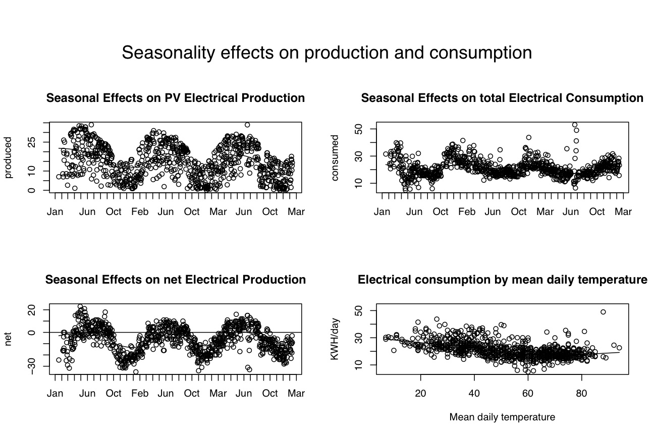
Upon inspection of these data, it seems as if during the first winter, there were some days with unusually high electrical consumption. Indeed, this was because the house was still under constrcution. We now redo the analysis with just days with consumption < 40 KWH/day. This makes use of the 'subset' command. However, we also notice that we had very high demand in July of 2005. This was due to about 6 days of air conditioning! We should include these data
normal=subset(electric,(consumed<40) |as.POSIXlt(date)$year>103 )       #select those days with more typical power consumption or after 2003
detach(electric)                         #release the names in this data frame to use the next one

attach(normal)       #use the names in the new data frame

#plot 4 different panels -- energy produced, consumed, net as function of date, consumption by temperature

smooth.value = 3/10                   #allows us to experiment with different smoothing parameters in lowess


plot.new()                               #start a new plot
                                        #set parameters for this graph
par(omi=c(0,0,1,0) )                      #set the size of the outer margins
par(mfrow=c(2,2))                        #number of rows and columns to graph

plot(date,produced,xaxt="n")          #don't plot the x axis
axis.POSIXct(1, at=seq(daterange[1], daterange[2], by="month"), format="%b") #label the x axis by months
lines(lowess(date,produced, f=smooth.value))   #lowess smooth with 30% window
title(main="Seasonal Effects on PV Electrical Production")

plot(date,consumed,xaxt="n")          #don't plot the x axis
axis.POSIXct(1, at=seq(daterange[1], daterange[2], by="month"), format="%b") #label the x axis by months
lines(lowess(date,consumed, f=smooth.value))   #lowess smooth with 30% window
title(main="Seasonal Effects on total Electrical Consumption")

net=produced-consumed     #net electrical production
plot(date,net,xaxt="n")          #don't plot the x axis
axis.POSIXct(1, at=seq(daterange[1], daterange[2], by="month"), format="%b") #label the x axis by months
lines(lowess(date,net, f=smooth.value))   #lowess smooth with 30% window
title(main="Seasonal Effects on net Electrical Production")
abline(h=0)

plot(temp1,consumed,main="Electrical consumption by mean daily temperature",xlab="Mean daily temperature",ylab="KWH/day")
lines(lowess.na(temp1,consumed,f=smooth.value))

mtext("Seasonality effects on production and consumption",3,outer=TRUE,line=1,cex=1.5)    #note that we seem to add the global title last
                     #cex = character expansion factor

plot.3=recordPlot()   #save this one before redoing with a different smooth value
smooth.value=.5
We can examine the effects of different levels of smoothing either by doing different graphs and saving them, or by plotting multiple smooths on each graph. Lets try multiple smoothing functions.
plot.new()                               #start a new plot
                                        #set parameters for this graph
par(omi=c(0,0,1,0) )                      #set the size of the outer margins
par(mfrow=c(2,2))                        #number of rows and columns to graph

plot(date,produced,xaxt="n")          #don't plot the x axis
axis.POSIXct(1, at=seq(daterange[1], daterange[2], by="month"), format="%b") #label the x axis by months
lines(lowess(date,produced, f=.25))   #lowess smooth with 25% window
lines(lowess(date,produced, f=1/3))   #lowess smooth with 33% window
lines(lowess(date,produced, f=.5))   #lowess smooth with 50% window
lines(lowess(date,produced, f=2/3))   #lowess smooth with 66% window
title(main="Analysis of Seasonal Effects on PV Electrical Production")

plot(date,consumed,xaxt="n")          #don't plot the x axis
axis.POSIXct(1, at=seq(daterange[1], daterange[2], by="month"), format="%b") #label the x axis by months
lines(lowess(date,consumed, f=.25))   #lowess smooth with 25% window
lines(lowess(date,consumed, f=1/3))   #lowess smooth with 33% window
lines(lowess(date,consumed, f=.5))   #lowess smooth with 50% window
lines(lowess(date,consumed, f=2/3))   #lowess smooth with 66% window
title(main="Analysis of Seasonal Effects on total Electrical Consumption")

net=produced-consumed     #net electrical production
plot(date,net,xaxt="n")          #don't plot the x axis
axis.POSIXct(1, at=seq(daterange[1], daterange[2], by="month"), format="%b") #label the x axis by months
lines(lowess(date,net, f=.25))   #lowess smooth with 25% window
lines(lowess(date,net, f=1/3))   #lowess smooth with 33% window
lines(lowess(date,net, f=.5))   #lowess smooth with 50% window
lines(lowess(date,net, f=2/3))   #lowess smooth with 66% window
title(main="Analysis of Seasonal Effects on net Electrical Production")
abline(h=0)

plot(temp1,consumed,main="Electrical consumption by mean daily temperature",xlab="Mean daily temperature",ylab="KWH/day")
lines(lowess.na(temp1,consumed,f=.25))
lines(lowess.na(temp1,consumed,f=1/3))
lines(lowess.na(temp1,consumed,f=.5))
lines(lowess.na(temp1,consumed,f=2/3))

mtext("Analysis of seasonality effects on production and consumption\r with 4 levels of smoothing",3,outer=TRUE,line=1,cex=1.5)    #note that we seem to add the global title last
                     #cex = character expansion factor
This results in the following 4 (messy) plots:
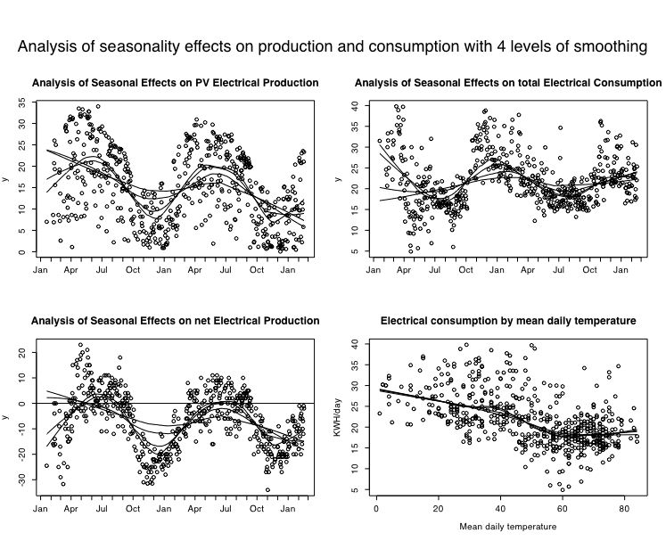
We would expect a seasonality effect in PV production, but why is there one for consumption? After examining the relationship between external temperature and consumption several hypotheses are likely. Although after one year I had thought this relationship was due to the use of electric pumps to deliver the radiant heat, after another winter's analysis, I believe this was due to overreliance on internal air circulation using HVAC equipment (as advised by an incompetent Heating Contractor) rather than the more appropriate use of an Energy Recovery Ventilation (HRV) system. Based upon the data from the first winter, we stopped using the HVAC system and used the ERV system in the second winter. Notice the decreased in energy consumption. In fact, the relationship is reduced across the years.
Another source of electrical consumption is driving a pump to circulate hot water (from a hot water solar system) to heat a small exercise pool. This can be seen from the plot of consumption by hours of heating, as well as the relationship between external temperature and kwh consumption as a function of hours of heating (a Coplot)
plot(poolheat,consumed,main="Effect of external temperature on electrical Consumption")
abline(lm(consumed~poolheat,data=normal))

 coplot(consumed~mean|poolheat,panel = panel.smooth)

 model=lm(consumed~mean+poolheat)
 model=lm(consumed~mean)


oneday=subset(normal,days==1)
detach(normal)
attach(oneday)
par(mfrow=c(2,1))
plot(poolheat,deltaheat,main="change in temperature as a function of hours of heating",ylab="change in temperature",xlab="hours of heating")
mod1=lm(deltaheat~poolheat)
abline(mod1)    #put the regression line in
plot(poolheat,consumed,main="electrical consumption as a function of hours of heating pool",ylab="KWH/day",xlab="Hours of pool heat")
mod2=lm(consumed~poolheat)
abline(mod2)
mtext("Effect of solar pool heating on pool heat and electrical consumption",3,outer=TRUE,line=1,cex=1.5)    #note that we seem to add the global title last
                     #cex = character expansion factor
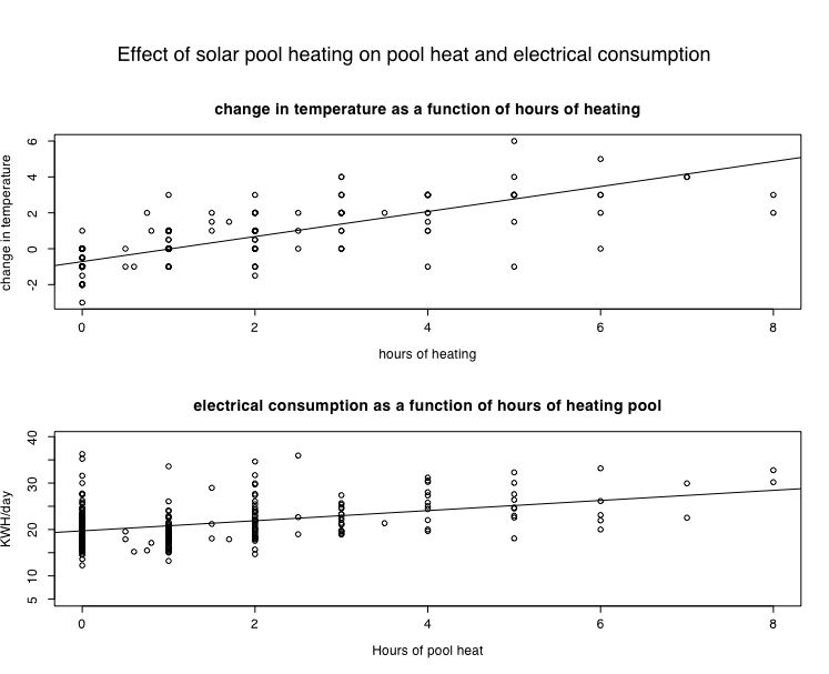
The strength of the relationship may be determined by examing the R-square of the regression which in the first case (hours of heating and change in temperature) is quite strong. Although the relationship is not as strong, the effect of running the pump on power consumption suggests that one hour of operation leads to about an additional KWH of power consumption.
summary(mod1)

Call:
lm(formula = deltaheat ~ poolheat)

Residuals:
     Min       1Q   Median       3Q      Max
-3.76586 -0.37228  0.02131  0.71810  3.23414

Coefficients:
            Estimate Std. Error t value Pr(>|t|)
(Intercept) -0.71810    0.08057  -8.912   <2e-16 ***
poolheat     0.69679    0.03708  18.791   <2e-16 ***
---
Signif. codes:  0 `***' 0.001 `**' 0.01 `*' 0.05 `.' 0.1 ` ' 1

Residual standard error: 1.009 on 254 degrees of freedom
Multiple R-Squared: 0.5816,	Adjusted R-squared:  0.58
F-statistic: 353.1 on 1 and 254 DF,  p-value: < 2.2e-16


summary(mod2)
summary(mod2)

Call:
lm(formula = consumed ~ poolheat)

Residuals:
    Min      1Q  Median      3Q     Max
-7.5670 -3.0012 -0.6728  2.2919 16.5615

Coefficients:
            Estimate Std. Error t value Pr(>|t|)
(Intercept)  19.7089     0.3291  59.880  < 2e-16 ***
poolheat      1.0901     0.1515   7.196 6.96e-12 ***
---
Signif. codes:  0 `***' 0.001 `**' 0.01 `*' 0.05 `.' 0.1 ` ' 1

Residual standard error: 4.121 on 254 degrees of freedom
Multiple R-Squared: 0.1694,	Adjusted R-squared: 0.1661
F-statistic: 51.79 on 1 and 254 DF,  p-value: 6.956e-12
Finally, lets try to get some monthly statistics. My solution to doing this sort is a kludge, but works.
month.year <- function (x) {12*(as.POSIXlt(x)$year-103)+as.POSIXlt(x)$mon+1} #months are mod 12 and normally range from 0-11.  this makes them go to 1-12

#attach(normal)          #get the cleaned data
month <- month.year(date) #months start at January 2003 and add from then

mean.produced=tapply(produced,month,mean)  #apply the mean function to amount produced each month
sd.produced=tapply(produced,month,sd)
mean.consumed <- tapply(consumed,month,mean)
sd.consumed <- tapply(consumed,month,sd)
months <- month.name   #names from January to December
for (i in 1 : length(mean.consumed)) {month.observed[i]<- as.numeric(names(mean.consumed[i]))%%12} #first get the months as numbers 0-11
month.observed[month.observed==0]<-12   # make the decembers 12 instead of 0
month.names <- months[as.numeric(month.observed)]

stats <- data.frame(mean.produced,sd.produced,mean.consumed,sd.consumed,month=month.names)
print(stats,digits=3)


#see also month.name and month.abb  for convenient use of months


#gives this output
   mean.produced sd.produced mean.consumed sd.consumed     month
2           7.02          NA          31.5          NA  February
3          14.75        7.44          27.8        4.34     March
4          19.70        9.18          29.9        7.34     April
5          20.76        9.62          15.4        6.78       May
6          24.72        7.45          17.8        5.13      June
7          21.08        7.42          18.9        5.22      July
8          20.19        5.57          17.4        1.96    August
9          17.57        6.63          15.0        3.05 September
10         14.76        5.92          17.7        2.72   October
11          6.69        3.73          26.7        4.07  November
12          7.51        4.49          32.3        4.05  December
13          6.50        5.03          28.1        4.11   January
14          8.26        6.10          26.7        4.62  February
15         12.41        6.08          26.2        5.26     March
16         22.58        5.40          24.1        5.01     April
17         18.49        7.42          21.1        3.86       May
18         20.90        6.86          20.0        3.94      June
19         19.78        6.57          17.6        2.19      July
20         17.79        7.25          18.9        3.98    August
21         19.56        3.58          18.1        2.27 September
22         12.27        7.19          17.7        2.64   October
23          6.98        4.94          23.0        5.52  November
24          6.71        3.95          25.8        6.23  December
25          5.97        5.32          24.8        3.65   January
26          9.28        6.33          21.2        3.23  February
27         14.17        6.36          21.3        3.91     March
28         20.19        6.69          18.3        2.94     April
29         18.60        7.49          16.3        2.84       May
30         22.06        5.14          17.6        4.14      June
31         20.42        6.90          21.7       15.46      July
32         20.96        4.35          16.5        1.81    August
33         10.56        7.17          17.1        2.33 September
34         10.25        5.70          18.1        3.14   October
35          8.63        5.22          22.0        2.72  November
36          5.66        5.09          23.4        3.76  December
37          7.31        5.30          23.5        4.16   January
38         10.74        5.46          23.6        3.46  February
In addition to plotting LOWESS smooths, we can also organize the date by months and do graphical analyses of monthly data. This uses the POSIXlt function to give us the numerical month.
Here are the results in boxplot form.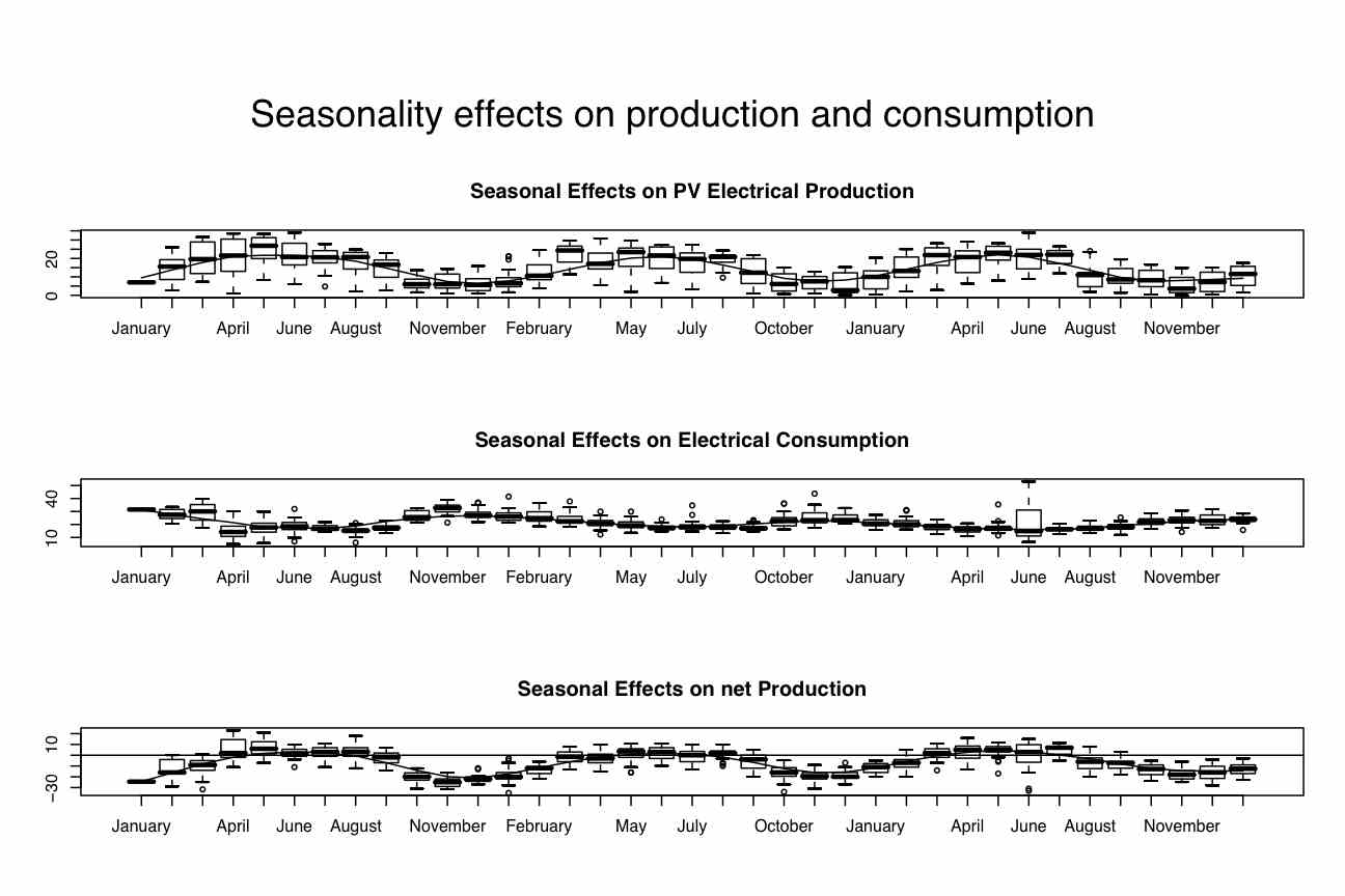
# as.POSIXlt(date)$mon #gives the months in numeric order mod 12 with January = 0 and December = 11
par(mfrow=c(3,1))
bproduced=boxplot(produced~month.year(date),names=month.names,data=normal ) #show the graph and save the data in bc
title(main="Seasonal Effects on PV Electrical Production",cex=1.5)
lines(lowess(bproduced$stats[3,],f=1/5)) #add a smooth to the box plot
bconsumed<-boxplot(consumed~month.year(date),names=month.names,data=normal )
title(main="Seasonal Effects on Electrical Consumption",cex=1.5)
lines(lowess(bconsumed$stats[3,],f=1/6))
bnet<-boxplot(net~month.year(date),names=month.names,data=normal )
title(main="Seasonal Effects on net Production",cex=1.5)
abline(h=0)
lines(lowess(bnet$stats[3,],f=1/6))
mtext("Seasonality effects on production and consumption",3,outer=TRUE,line=1,cex=1.5) #cex = character expansion factor
# as.POSIXlt(date)$mon #gives the months in numeric order mod 12 with January = 0 and December = 11
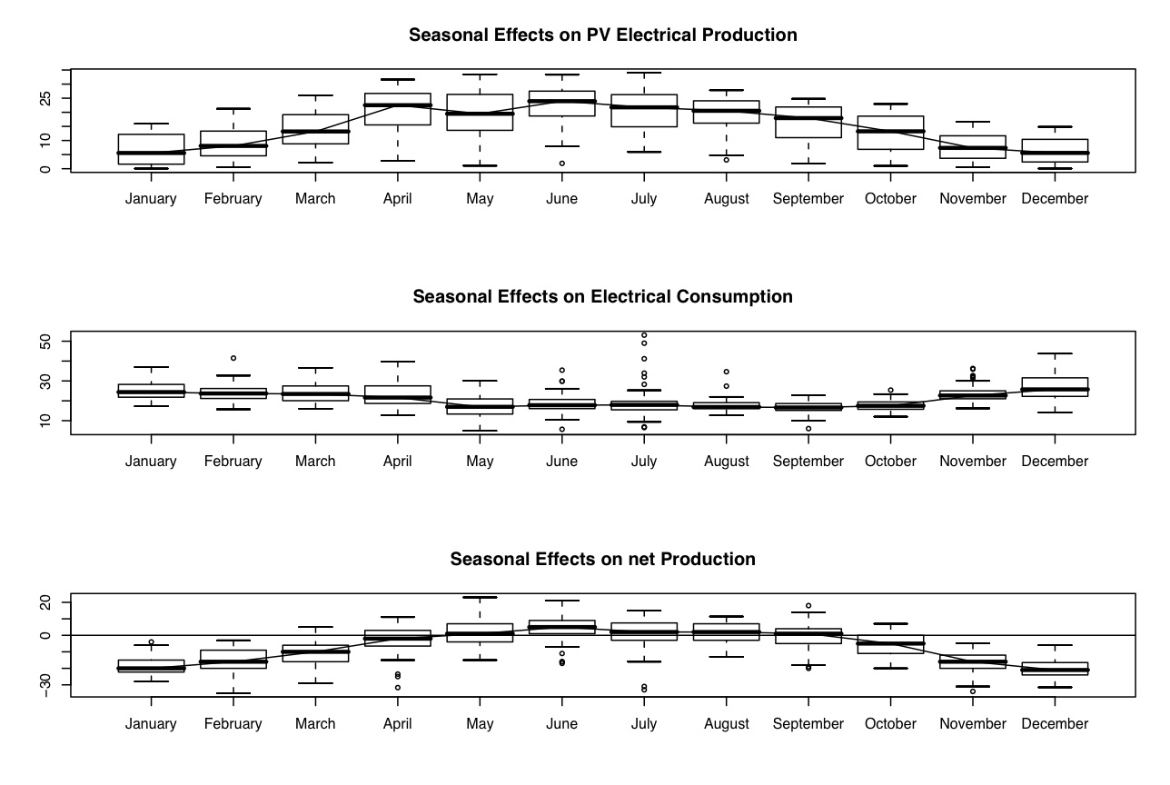
#now do it for months collapsed across years
par(mfrow=c(3,1))
bproduced=boxplot(produced~ as.POSIXlt(date)$mon,names=months ,data=normal ) #show the graph and save the data in bc
title(main="Seasonal Effects on PV Electrical Production",cex=1.5)
lines(lowess(bproduced$stats[3,],f=1/5)) #add a smooth to the box plot
bconsumed<-boxplot(consumed~ as.POSIXlt(date)$mon,names=months,data=normal )
title(main="Seasonal Effects on Electrical Consumption",cex=1.5)
lines(lowess(bconsumed$stats[3,],f=1/6))
bnet<-boxplot(net~ as.POSIXlt(date)$mon,names=months,data=normal )
title(main="Seasonal Effects on net Production",cex=1.5)
abline(h=0)
lines(lowess(bnet$stats[3,],f=1/6))
mtext("Seasonality effects on production and consumption",3,outer=TRUE,line=1,cex=1.5) #cex = character expansion factor
Monthly box plot
 par(mfrow=c(3,1))
bproduced=boxplot(produced~month.year(date),data=normal,names=month.names )   #show the graph and save the data in bc
title(main="Seasonal Effects on PV Electrical Production",cex=1.5)
lines(lowess(bproduced$stats[3,],f=1/5))    #add a smooth to the box plot

bconsumed<-boxplot(consumed~month.year(date),names=month.names,data=normal )
title(main="Seasonal Effects on Electrical Consumption",cex=1.5)
lines(lowess(bconsumed$stats[3,],f=1/6))

bnet<-boxplot(net~month.year(date),names=month.names,data=normal )
title(main="Seasonal Effects on net Production",cex=1.5)
abline(h=0)
lines(lowess(bnet$stats[3,],f=1/6))
mtext("Seasonality effects on production and consumption",3,outer=TRUE,line=1,cex=1.5)    #cex = character expansion factor
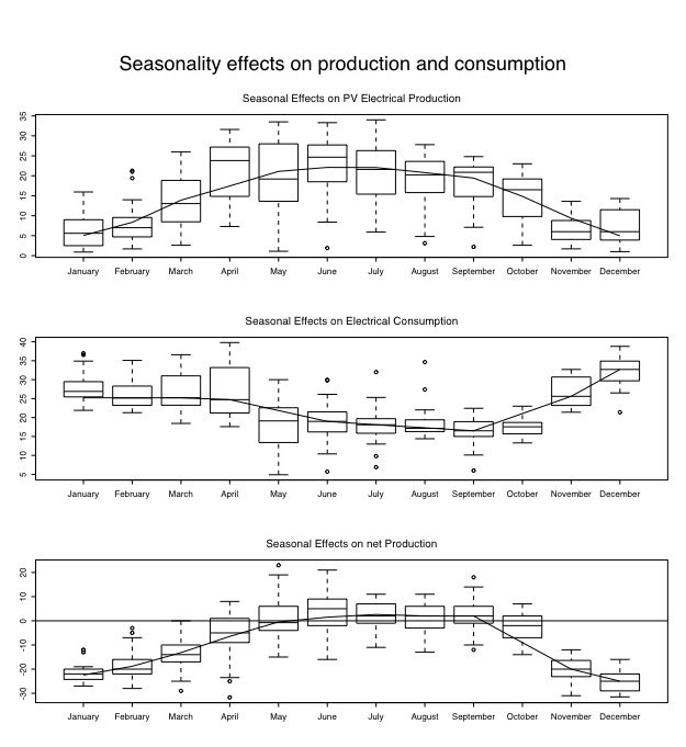
The fitted line going through the medians is a lowess smooth. Note that we need to run the box plots first to get the appropriate statistics. Further note that the fraction of data included in the smooth function = 1/3. This recognizes the summer months are net production months better than a larger fraction.
new.plot()
par(mfrow=c(1,1))

plot(bproduced$stats[3,],xaxt="n",xlab="Time of Year",ylab="KWH/day",ylim=c(-25,35),type="b",lwd=4)
axis(1,labels=c("February","April","June","August","October","December"))
#lines(lowess(bproduced$stats[3,]))


points(bconsumed$stats[3,],xaxt="n",type="b",lwd=2,col="red")
#lines(lowess(bconsumed$stats[3,]))


points(bnet$stats[3,],xaxt="n",type="b")
axis(1,labels=c("February","April","June","August","October","December"))
#lines(lowess(bnet$stats[3,]))
abline(h=0)
mtext("Production and consumption vary over the year ",3,outer=TRUE,line=1,cex=1.5)    #note that we seem to add the global title last
                     #cex = character expansion factor
percent=100*produced/consumed


bpercent=boxplot(percent~(as.POSIXlt(date)$mon+as.POSIXlt(date)$year),names=month.names )   #show the graph and save the data in bc
plot(bpercent$stats[3,],xaxt="n",xlab="Time of Year",ylab="% of demand",type="b",ylim=c(0,150),lwd=2)
abline(h=100)
axis(1,labels=c("February","April","June","August","October","December"))
title(main="Annual electrical production is 70% of total demand")
It is also possible to plot multiple points and fits on the same graph. Consider a plot of solar output/solar slate as a function of roof pitch and orientation.
plot.new()                               #start a new plot
                                        #set parameters for this graph
par(omi=c(0,0,1,0) )                      #set the size of the outer margins
par(mfrow=c(1,1))                        #number of rows and columns to graph

plot(date,belvederewatts,xaxt="n",pch=19,ylab="watt hours")          #don't plot the x axis
axis.POSIXct(1, at=seq(daterange[1], daterange[2], by="month"), format="%b") #label the x axis by months
lines(lowess(date,belvederewatts, f=smooth.value),lty=1)   #lowess smooth with 30% window
points(date,garagewatts,pch=21)
lines(lowess(date,garagewatts,f=smooth.value),lty=2)
points(date,midwatts,pch=23)
lines(lowess(date,midwatts,f=smooth.value),lty=3)
title(main="Seasonal Effects on PV Electrical Production (per slate/day)")


plot(belvederewatts,garagewatts,pch=19)
points(belvederewatts,midwatts,pch=21)
abline(0,1)
Now, to calculate the effeciency of the converter, we can compare net consumption to production. We need to select days where we were not heating the pool.
part of a short guide to R
Version of Feb 10, 2006
William Revelle
Northwestern University