Table of Contents
Introduction
General Comments
Data Manipulation
Graphic displays
Multivariate Analysis
- alpha reliability
- Factor Analysis
- Very Simple Structure
- Finding Omega for reliability
- Cluster analysis
- Multidimensional Scaling
- Structural Equation Modeling
- Item Response Theory
- Data simulation
Adding new functions/packages
- e.g., the psych package
Partial list of useful commands
Short Course lecture notes
How To tutorials include
Additional Resources from the web
- Resources for R Sara Weston/Debbie Yee
Using R for psychological research
A simple guide to an elegant language
This is one page of a series of tutorials for using R in psychological research. Much of material has also covered been covered in number of short courses or in a set of tutorials for specific problems. This page has been lightly edited in September 2020, but is generally very out of date. I recommend the tutorials or the various short courses.
Introduction to R
(For two very abbreviated, and very out of date, forms of this guide meant to help students do basic data analysis in a personality research course, see a very short guide. In addition, a short guide to data analysis in a research methods course offers some more detail on graphing. These two will be updated soon.)
Get the definitive Introduction to R written by members of the R Core Team.
There are many possible statistical programs that can be used in psychological research. They differ in multiple ways, at least some of which are ease of use, generality, and cost. Some of the more common packages used are Systat, SPSS, and SAS. These programs have GUIs (Graphical User Interfaces) that are relatively easy to use but that are unique to each package. These programs are also very expensive and limited in what they can do. Although convenient to use, GUI based operations are difficult to discuss in written form. When teaching statistics or communicating results to others, it is helpful to use examples that may be used by others using different computing environments and perhaps using different software. This set of brief notes describes an alternative approach that is widely used by practicing statisticians, the statistical environment R. This is not meant as a user's guide to R, but merely the first step in guiding people to helpful tutorials. I hope that enough information is provided in this brief guide to make the reader want to learn more. (For the impatient, an even briefer guide to analyzing data for personality research is also available.)
It has been claimed that "The statistical programming language and computing environment S has become the de-facto standard among statisticians. The S language has two major implementations: the commercial product S-PLUS, and the free, open-source R. Both are available for Windows and Unix/Linux systems; R, in addition, runs on Macintoshes." From John Fox's short course on S and R.
The R project, based upon the S and S+ stats packages, has developed an extremely powerful set of "packages" that operate within one program. Although described as merely "an effective data handling and storage facility [with] a suite of operators for calculations on arrays, in particular, matrices" R is, in fact, a very useful interactive package for data analysis. When compared to most other stats packages used by psychologists, R has at least three compelling advantages: it is free, it runs on multiple platforms (e.g., Windows, Unix, Linux, and Mac OS X), and combines many of the most useful statistical programs into one quasi integrated program..
More important than the cost is the fact that R is open source. That is, users have the ability to inspect the code to see what is actually being done in a particular calculation. (R is free software as part of the GNU Project. That is, users are free to use, modify, and distribute the program, within the limits of the GNU non-license) The program itself and detailed installation instructions for Linux, Unix, Windows, and Macs are available through CRAN (Comprehensive R Archive Network). Somewhat pedantic instructions for installing R are in my tutorial Getting Started with R and the psych package.
Although many run R as a language and programming environment, there are Graphical User Interfaces (GUIs) available for PCs, Linux and Macs. See for example, R Commander by John Fox, RStudio and R-app for the Macintosh developed by Stefano M. Iacus and Simon Urbanek. Compared to the basic PC environment, the Mac GUI is to be preferred. Many users find RStudio to be the preferred environment. It provides the same user experience on PCs and on Macs.
A note on the numbering system: The R-development core team releases an updated version of R about every six months. The current version is 4.0.2 was released in June, 2020.
R is an integrated, interactive environment for data manipulation and analysis that includes functions for standard descriptive statistics (means, variances, ranges) and also includes useful graphical tools for Exploratory Data Analysis. In terms of inferential statistics R has many varieties of the General Linear Model including the conventional special cases of Analysis of Variance, MANOVA, and linear regression.
What makes R particularly powerful is that statisticians and statistically minded people around the world have contributed more than 16,200 packages to the R Group and maintain a very active news group offering suggestions and help. The growing collection of packages and the ease with which they interact with each other and the core R is perhaps the greatest advantage of R. Advanced features include correlational packages for multivariate analyses including Factor and Principal Components Analysis, and cluster analysis. Advanced multivariate analyses packages that have been contributed to the R-project include at least three for Structural Equation Modeling (sem, lavaan, and Open-Mx), Multi-level modeling (also known as Hierarchical Linear Modeling and referred to as non linear mixed effects in the nlme4 package) and taxometric analysis. All of these are available in the free packages distributed by the R group at CRAN. Many of the functions described in this tutorial are incorporated into the psych package. Other packages useful for psychometrics are described in a task-view at CRAN. In addition to be a environment of prepackaged routines, R is a interpreted programming language that allows one to create specific functions when needed.
In addition to be a package of routines, R is a interpreted programming language that allows one to create specific functions when needed. This does not require great skills at programming and allows one to develop short functions to do repetitive tasks.
R is also an amazing program for producing statistical graphics. A collection of some of the best graphics was available at addictedtoR with a complete gallery of thumbnail of figures. This seems to have vanished. However, the site R graph Gallery is worth visiting if you are willing to ignore the obnoxious ads.
An introduction to R is available as a pdf or as a paper back. It is worth reading and rereading. Once R is installed on your machine, the introduction may be obtained by using the help.start command. More importantly for the novice, a number of very helpful tutorials have been written for R. (e.g., the tutorial by John Verzani to help one teach introductory statistics and learn R at the same time--this has now been published as a book, but earlier versions are still available online), or (by Jonathan Baron and Yuelin Li) to use R in the Psychology lab. The Baron and Li tutorial is the most useful for psychologists trying to learn R. Another useful resource is John Fox's short course on R. For a more complete list of brief (<100 pages) and long( > 100 pages) tutorials, go to the contributed section of the CRAN.
There are a number of "reference cards" also known as "cheat sheets" that provide quick summaries of commands.
- Jonathan Baron's one pager
- Tom Short's four pager
- Paul Torfs and Claudia Brauer not so short introduction
To download a copy of the software, go to the download section of the cran.r-project.org site. A detailed pdf of how to download R and some of the more useful packages is available as part of the personality-project.
This set of notes relies heavily on "An introduction to R" by Venables, Smith and the R Development Core Team, the very helpful Baron and Li guide and the teaching stats page of John Verzani. Their pages were very useful when I started to learn R. There is a growing number of text books that introduce R. One of the classics is "Modern Applied Statistics with S" by Brian D. Ripley and William N. Venables. For the psychometrically minded, my psychometrics text (in progress) has all of its examples in R.
The R help listserve is a very useful source of information. Just lurking will lead to the answers for many questions. Much of what is included in this tutorial was gleaned from comments sent to the help list. The most frequently asked questions have been organized into a FAQ. The archives of the help group are very useful and should be searched before asking for help. Jonathan Baron maintains a searchable database of the help list serve. Before asking for help, it is important to read the posting guide as well as “How to Ask Questions the Smart Way”.
For a thoughtful introduction to R for SPSS and SAS users, see the tutorials developed at the University of Tennessee by Bob Muenchen. For a comparison of what is available in R to what is available in SPSS or SAS, see his table comparing the features of R to SPSS. He compares a number of languages for data science.
General Comments
R is not overly user friendly (at first). Its error messages are at best cryptic. It is, however, very powerful and once partially mastered, easy to use. And it is free. Even more important than the cost is that it is an open source language which has become the lingua franca of statistics and data analysis. That is, as additional modules are added, it becomes even more useful. Modules included allow for multilevel (hierarchical) linear modeling, confirmatory factor analysis, etc. I believe that it is worth the time to learn how to use it. J. Baron and Y. Li's guide is very helpful. They include a one page pdf summary sheet of commands that is well worth printing out and using. A three page summary sheet of commands is available from Rpad.
Using R in 12 simple steps for psychological research
(These steps are not meant to limit what can be done with R, but merely to describe how to do the analysis for the most basic of research projects and to give a first experience with R).
- Install R on your computer or go to a machine that has it.
- Download the psych package as well as other recommended packages from CRAN using the install.packages function, or using the package installer in the GUI. To get packages recommended for a particular research field, use the ctv package to install a particular task view. Note, these first two steps need to be done only once!
- Activate the psych package or other desired packages using e.g., library(psych). This needs to be done every time you start R. Or, it is possible to modify the startup parameters for R so that certain libraries are loaded automatically.
- Enter your data using a text editor and save as a text file (perhaps comma delimited if using a spreadsheet program such as Excel or OpenOffice)
- Read the data file or copy and paste from the clipboard (using, e.g., read.clipboard).
- Find basic descriptive statistics (e.g., means, standard deviations, minimum and maxima) using describe.
- Prepare a simple descriptive graph (e.g, a box plot) of your variables.
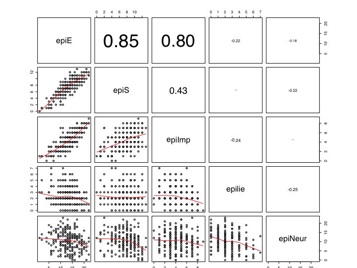
- Find the correlation matrix to give an overview of relationships (if the number is not too great, a scatter plot matrix or SPLOM plot is very useful, this can be done with pairs.panels.
- If you have an experimental variable, do the appropriate multiple regression using standardized or at least zero centered scores.
- If you want to do a factor analysis or principal components analysis, use the fa or principal functions.
- To score items and create a scale and find various reliability estimates, use score.items and perhaps omega.
- Graph the results.
Getting started
Installing R on your computer
Although it is possible that your local computer lab already has R, it is most useful to do analyses on your own machine. In this case you will need to download the R program from the R project and install it yourself. Using your favorite web browser, go to the R home page at https://www.r-project.org and then choose the Download from CRAN (Comprehensive R Archive Network) option. This will take you to list of mirror sites around the world. You may download the Windows, Linux, or Mac versions at this site. For most users, downloading the binary image is easiest and does not require compiling the program. Once downloaded, go through the install options for the program. If you want to use R as a visitor it is possible to install R onto a “thumb drive” or “memory stick” and run it from there. (See the R for Windows FAQ at CRAN).
Packages and Task Views
One of the great strengths of R is that it can be supplemented with additional programs that are included as packages using the package manager. (e.g., sem or OpenMX do structural equation modeling) or that can be added using the source command. Most packages are directly available through the CRAN repository. Others are available at the BioConductor (https://www.bioconductor.org) repository. Yet others are available at “other” repositories. The psych package (Revelle, 2020) may be downloaded from CRAN or from the https: //personality-project.org/r repository.
The concept of a “task view” has made downloading relevant packages very easy. For instance, the install.views("Psychometrics") command will download over 50 packages that do various types of psychometrics. To install the Psychometrics task view will take a few minutes, so you might want to do this when you have some free time.
install.packages("ctv")
library(ctv)
install.views("Psychometrics")
For any other than the default packages to work, you must activate it by either using the Package Manager or the library command, e.g.,
library(psych)
library(sem)
entering ? the name of a package (e.g.,)
?psych
will give a list of the functions available in that package (e.g., psych) package as well as an overview of their functionality.
objects(package:psych)
will list the functions available in a package (in this case, psych).
If you routinely find yourself using the same packages everytime you use R, you can modify the Startup process by specifying what should happen .First. Thus, if you always want to have psych available,
.First <- function(library(psych))
and then when you quit, use the save workspace option.
Help and Guidance
R is case sensitive and does not give overly useful diagnostic messages. If you get an error message, don’t be flustered but rather be patient and try the command again using the correct spelling for the command. Issuing the up arrow command will let you edit the previous command.
When in doubt, use the help () function. This is identical to the ? function where function is what you want to know about. e.g.,
help(read.table)  #or
?read.table   #another way of asking for help
asks for help in using the read.table function. the answer is in the help window.
apropos("read") #returns all available functions with that term in their name.
RSiteSearch("read") #opens a webbrowser and searches voluminous files
RSiteSearch(“keyword”) will open a browser window and return a search for “keyword” in all functions available in R and the associated packages as well (if desired) the R-Help News groups.
All packages and all functions will have an associated help window. Each help window will give a brief description of the function, how to call it, the definition of all of the available parameters, a list (and definition) of the possible output, and usually some useful examples. One can learn a great deal by using the help windows, but if they are available, it is better to study the package vignette.
Package vignettes
All packages have help pages for each function in the package. These are meant to help you use a function that you already know about, but not to introduce you to new functions. An increasing number of packages have a package vignettes that give more of an overview of the program than a detailed description of any one function. These vignettes are accessible from the help window and sometimes as part of the help index for the program. The seven vignettes for the psych package are also available from the personality project web page. (An introduction to the psych package, a "How to" get started , how to find the omega coefficients, how to score scales from items, how to do mediation and moderation analysis and how to do factor analysis, and Using the psych package as a front end to the sem package).
Commands are entered into the "R Console" window. You can add a comment to any line by using a #. The Mac version has a text editor window that allows you to write, edit and save your commands. Alternatively, if you use a normal text editor (As a Mac user, I use BBEDIT, PC users can use Notepad), you can write out the commands you want to run, comment them so that you can remember what they do the next time you run a similar analysis, and then copy and paste into the R console.
Although being syntax driven seems a throwback to an old, pre Graphical User Interface type command structure, it is very powerful for doing production statistics. Once you get a particular set of commands to work on one data file, you can change the name of the data file and run the entire sequence again on the new data set. This is is also very helpful when doing professional graphics for papers. In addition, for teaching, it is possible to prepare a web page of instructional commands that students can then cut and paste into R to see for themselves how things work. That is what may be done with the instructions on this page. It is also possible to write text in latex with embedded R commands. Then executing the Sweave function on that text file will add the R output to the latex file. This almost magical feature allows rapid integration of content with statistical techniques. More importantly, it allows for "reproducible research" in that the actual data files and instructions may be specified for all to see. All of the vignettes listed above use that technique.
As you become more adept in using R, you will be tempted to enter commands directly into the console window. I think it is better to keep (annotated) copies of your commands to help you next time.
If you are using R studio, then create a Markdown document to record and annotate your commands.
Command syntax tends to be of the form:
variable = function (parameters) or
variable <- function (parameters) the = and the <- symbol imply replacement, not equality
the preferred style is to use the <- symbol to avoid confusion.
elements of arrays are indicated within brackets [ ]
This guide assumes that you have installed a copy of R onto your computer and you are trying out the commands as you read through this. (Not necessary, but useful.)
Help and Guidance
For a list of all the commands that use a particular word, use the apropos () command:
apropos(table)  #lists all the commands that have the word "table" in them

apropos(table)
 [1]"ftable"              "model.tables" "pairwise.table"   "print.ftable"        "r2dtable"
 [6]"read.ftable"         "write.ftable" ".__C__mtable"     ".__C__summary.table" ".__C__table"
[11]"as.data.frame.table" "as.table"     "as.table.default" "is.table"           "margin.table"
[16]"print.summary.table" "print.table"  "prop.table"       "read.table"       "read.table.url"
[21]"summary.table"       "table"        "write.table"      "write.table0"
For more complicated functions (e.g., plot(), lm()) the help function shows very useful examples. A very nice example is demo(graphics) which shows many of the complex graphics that are possible to do. demo(lm.glm) gives many examples of the linear model/general linear model.
Entering or getting the data
There are multiple ways of reading data into R.
From a text file
For very small data sets, the data can be directly entered into R. For more typical data sets, it useful to use a simple text editor or a spreadsheet program (e.g., Excel or OpenOffice). You can enter data in a tab delimted form with one variable per column and columns labeled with unique name. A numeric missing value code (say -999) is more convenient than using "." ala Systat. To read the data into a rows (subjects) by columns (variables) matrix use the read.table command.
A very useful command, for those using a GUI is file.choose() which opens a typical selection window for choosing a file.
#specify the name and address of the remote file

datafilename <- file.choose()     # use the OS to find the file

#e.g.,  datafilename <- "Desktop/epi.big5.txt"  #locate the local directory

person.data  <- read.table(datafilename,header=TRUE)  #read the data file

#Alternatively, to read in a comma delimited file:
#person.data  <- read.table(datafilename,header=TRUE,sep=",")
From the clipboard
For many problems you can just cut and paste from a spreadsheet or text file into R using the read.clipboard command from the psychTools package.
 my.data <- read.clipboard()      #or
 my.data <- read.clipboard.csv()  #if comma delimited
 my.data <- read.clipboard.tab()  #if tab delimited (e.g., from Excel
Files can be comma delimited (csv) as well. In this case, you can specify that the seperators are commas. For very detailed help on importing data from different formats (SPSS, SAS, Matlab, Systat, etc.) see the data help page from Cran. The foreign package makes importing from SPSS or SAS data files fairly straightforward.
From the web
For teaching, it is important to note that it is possible to have the file be a remote file read through the web. (Note that for some commands, there is an important difference between line feeds and carriage returns. For those who use Macs as web servers, make sure that the unix line feed is used rather than old Mac format carriage returns.) For simplicity in my examples I have separated the name of the file to be read from the read.table command. These two commands can be combined into one. The file can be local (on your hard disk) or remote.
For most data analysis, rather than manually enter the data into R, it is probably more convenient to use a spreadsheet (e.g., Excel or OpenOffice) as a data editor, save as a tab or comma delimited file, and then read the data or copy using the read.clipboard() command. Most of the examples in this tutorial assume that the data have been entered this way. Many of the examples in the help menus have small data sets entered using the c() command or created on the fly.
Data input example
For the first example, we read data from a remote file server for several hundred subjects on 13 personality scales (5 from the Eysenck Personality Inventory (EPI), 5 from a Big Five Inventory (BFI), the Beck Depression Inventory, and two anxiety scales). The file is structured normally, i.e. rows represent different subjects, columns different variables, and the first row gives subject labels. (To read from a local file, we simply change the name of the datafilename.)
#specify the name and address of the remote file
datafilename <- "https://personality-project.org/r/datasets/maps.mixx.epi.bfi.data"
#datafilename <- "Desktop/epi.big5.txt"  #read from local directory  or
# datafilename <- file.choose()     # use the OS to find the file
#in all cases
person.data  <- read.table(datafilename,header=TRUE)  #read the data file

#Alternatively, to read in a comma delimited file:
#person.data  <- read.table(datafilename,header=TRUE,sep=",")


names(person.data)  #list the names of the variables
produces this output
> datafilename <- "https://personality-project.org/r/datasets/maps.mixx.epi.bfi.data"
> #datafilename <- "Desktop/epi.big5.txt"  #read from local directory
> #person.data  <- read.table(datafilename,header=TRUE)  #read the data file
> person.data <- read.file(datafilename)  #this assumes header information
> #Alternatively, to read in a comma delimited file:
> #person.data  <- read.table(datafilename,header=TRUE,sep=",")


> names(person.data)  #list the names of the variables
 [1] "epiE"     "epiS"     "epiImp"   "epilie"    "epiNeur"   "bfagree"  "bfcon"    "bfext"
 [9] "bfneur"   "bfopen"   "bdi"      "traitanx"  "stateanx"
The data are now in the data.table "person.data". Tables allow one to have columns that are either numeric or alphanumeric. To address a particular row (e.g., subject = 5) and column (variable = 7) you simplely enter the required fields:
person.data[5,8]         #the 5th subject, 8th variable  or
person.data[5,"bfext"]   #5th subject,  "Big Five Inventory - Extraversion" variable
#or
person.data[5,]         #To list all the data for a particular subject (e.g, the 5th subject)
person.data[5:10,]      #list cases 5 - 10
person.data[5:10,"bfext"]  #list  just the extraversion scores for subjects 5-10
person.data[5:10,4:8]      #list the 4th through 8th variables for subjects 5 - 10.
In order to select a particular subset of the data, use the subset function. The next example uses subset to display cases where the lie scale was pretty high
subset(person.data,epilie>6)    #print the data meeting the logical condition epilie>6
#also try
person.data[person.data["epilie"]>6,]
produces this output
epiE epiS epiImp epilie epiNeur bfagree bfcon bfext bfneur bfopen bdi traitanx stateanx
16    11    5      6      7      13     126    78   112     83    132   4       45       28
212    6    4      1      7       4     147   119   102     81    142   2       26       21
One can also selectively display particular columns meeting particular criteria, or selectively extract variables from a dataframe.
subset(person.data[,2:5],epilie>5 & epiNeur<3) #notice that we are taking the logical 'and'


 epiS epiImp epilie epiNeur
12    12      3      6       1
118    8      2      6       2

subset(person.data[,3:7], epilie>6 | epiNeur ==2 ) #do a logical 'or' of the two conditions

epi <- subset(data,select=epiE:epiNeur)  #select particular variables from a data frame
Reading data from SPSS or other stats programs
In addition to reading text files from local or remote servers, it is possible to read data saved in other stats programs (e.g., SPSS, SAS, Minitab). read commands are found in the package foreign. You will need to make it active first. However, many of the standard file types may be read directly using the read.file function from psychTools
datafilename <- "https://personality-project.org/r/datasets/finkel.sav"   #remote file

eli.data <- read.file(datafilename)
Data sets can be saved for later analyses using the save command and then reloaded using load. If files are saved on remote servers, use the load(url(remoteURLname)) command.
save(object,file="local name") #save an object (e.g., a correlation matrix) for later analysis
load(file)         	       #gets the object (e.g., the correlation matrix back)
load(url("https://personality-project.org/r/datasets/big5r.txt"))  #get the correlation matrix
Getting around in R
R is case sensitive so be careful when naming or calling functions and variables. Commands are entered in the command console and (at least for Macs), are colored blue while results in the results console are shown in black. Commands can be cut and pasted from a text editor (or from a browser if following along with examples) into the command console. Like Unix or OS X, using the up arrow shows previous commands.
It is a useful habit to be consistent in your own naming conventions. Some use lower case letters for variables, Capitalized for data frames, all caps for functions, etc. It is easier to edit your code if you are reasonably consistent. Comment your code as well. This is not just so others can use it, but so that you can remember what you did 6 months later.
ls() #shows the variables in the workspace
help (name) #provides help about a function "name"

? name #does the same

rm(variable) #removes that variable

rm(list = ls()) #removes all variables from the work space
attach("table") #makes the elements of "table" available to be called directly (make sure to always detach later.
#  The use of attach ... detach has become discouraged.

names(table) #what are the variables inside the table

variable <-c(value1,value2,value3 ...)   #assigns values to a variable.
 # column bind (combine) variables to make up a new array with these variables

newvariable <- cbind (variable1, variable2, variable3 ... variable n)


#  e.g.


ls()     #show the variables in the workspace


datafilename <- "https://personality-project.org/R/datasets/maps.mixx.epi.bfi.data"
person.data <-  read.file(datafilename)  #read the data file
names(person.data)  #list the names of the variables
colnames(person.data) #specify that you want the names of the columns

attach(person.data)      #make the separate variable available -- always do detach when finished.
             #The with construct is better.

new.epi <-  cbind(epiE,epiS,epiImp,epilie,epiNeur)       #form a new variable "epi"
epi.df <- data.frame(new.epi)      #actually, more useful to treat this variable as a data frame

bfi.df <- data.frame(cbind(bfext,bfneur,bfagree,bfcon,bfopen))
	#create bfi as a data frame as well

detach(person.data)   #  very important to detach after an attach
The use of the attach -- detach sequence has become less common and it is more common to use the with command. The syntax of this is clear
with(some data frame, { do the commands between the brackets} ) #and then close the parens
#alternatively:
with(person.data,{
    epi <-  cbind(epiE,epiS,epiImp,epilie,epiNeur)       #form a new variable "epi"
    epi.df <- data.frame(epi)      #actually, more useful to treat this variable as a data frame

bfi.df <- data.frame(cbind(bfext,bfneur,bfagree,bfcon,bfopen))
	#create bfi as a data frame as well
   epi.df <- data.frame(epi)      #actually, more useful to treat this variable as a data frame

bfi.df <- data.frame(cbind(bfext,bfneur,bfagree,bfcon,bfopen))
	#create bfi as a data frame as well

describe(bfi.df)
}  #end of the stuff to be done within the with command
)   #end of the with command
However, intermediate results created inside the with ( ) command are not available later. The with construct is more appropriate when doing some specific analysis.
However, this is R, so there is yet another way of doing this that is very understandable:
#alternatively:
epi.df <- data.frame(with(person.data,{ cbind(epiE,epiS,epiImp,epilie,epiNeur)}  )) #actually, more useful to treat this variable as a data frame

bfi.df <- data.frame(with(person.data,cbind(bfext,bfneur,bfagree,bfcon,bfopen)) )
	#create bfi as a data frame as well
   epi.df <- data.frame(epi)      #actually, more useful to treat this variable as a data frame
Yet another way to call elements of a variable is to address them directly, either by name or by location:
epi <-  person.data[c("epiE","epiS","epiImp","epilie","epiNeur") ]      #form a new variable "epi"
epi.df <- data.frame(epi)      #actually, more useful to treat this variable as a data frame

bfi.df <- data.frame(person.data[c(9,10,7,8,11)])   #create bfi as a data frame as well
It is also possible to edit the data:
ls()    #show the variables
y <- edit(person.data)
	#show the data.frame or matrix x in a text editor and save changes to y
fix(person.data)
	#show the data.frame or matrix x in a text editor
invisibible(edit(x))
        #creates an edit window without also printing to console -- directly make changes.
        #Similar to the most basic spreadsheet.  Very dangerous!
head(x)  #show the first few lines of a data.frame or matrix
tail(x)  #show the last few lines of a data.frame or matrix
str(x)  #show the structure of x
Data manipulation
The normal mathematical operations can be done on all variables. e.g.
attach(person.data)   #make the variables inside person data available
imp2 <- epiImp*epiImp    #square epiImp
si <- epiS+epiImp        #sum sociability and impulsivity
statetotrait <- stateanx/traitanx  #find the ratio of state to trait anxiety
})
weirdproduct <- epi*bfi     #multiply respective elements in two tables
meanimp <- mean(imp)
stdevimp <- sd(imp)
standarizedimp <- scale(imp,scale=TRUE)    #center and then divide by the standard deviation
detach(person.data)   #and make sure to detach the variable when you are finished with it
Logical operations can be performed. Two of the most useful are the ability to replace if a certain condition holds, and to find subsets of the data.
person.data[person.data == -9] <- NA
	#replace all cases where a particular code is observed with NA


males=subset(person.data |gender ==1)
	#x=subset(y|condition)
The power of R is shown when we combine various data manipulation procedures. Consider the problem of scoring a multiple choice test where we are interested in the number of items correct for each person. Define a scoring key vector and then score as 1 each item match with that key. Then find the number of 1s for each subject. We use the Iris data set as an example.
iris2 <- round(iris[1:10,1:4])   #get a sample data set
key <- iris2[1,]    #make up an arbitary answer key
score <- t(t( rowSums((iris2 == c(key[]))+0)))   #look for correct item and add them up
mydata <- data.frame(iris2,score)     #
key         #what is the scoring key
mydata      #show the data with the number of items that match the key
(Thanks to Gabor Grothendieck and R help for this trick. Actually, to score a multiple choice test, use score.multiple.choice in the psych package.)
Basic descriptive statistics
Back to Top Core R includes the basic statistical functions one would want to provide summaries of the data. The summary command is not particularly helpful and the mean, min, max, sum, etc commands will be of a complete data set, not a single column.
Many if not most psychologists will probably prefer the output provided by the describe function in the psych package:
describe(epi.df)
         var   n  mean   sd median trimmed  mad min max range  skew kurtosis   se
epiE      1 231 13.33 4.14     14   13.49 4.45   1  22    21 -0.33    -0.06 0.27
epiS      2 231  7.58 2.69      8    7.77 2.97   0  13    13 -0.57    -0.02 0.18
epiImp    3 231  4.37 1.88      4    4.36 1.48   0   9     9  0.06    -0.62 0.12
epilie    4 231  2.38 1.50      2    2.27 1.48   0   7     7  0.66     0.24 0.10
epiNeur   5 231 10.41 4.90     10   10.39 4.45   0  23    23  0.06    -0.50 0.32
Standardization and zero centering scale) that does this automatically
 epiz <- scale(epi)          #centers (around the mean) and scales by the sd
 epic <- scale(epi,scale=FALSE) #centers but does not Scale
Compare the two results. In the first, all the means are 0 and the sds are all 1. The second also has been centered, but the standard deviations remain as they were.
 describe(epiz)
 describe(epic)


 >  describe(epiz)
        var   n mean sd median trimmed  mad   min  max range  skew kurtosis   se
epiE      1 231    0  1   0.16    0.04 1.08 -2.98 2.10  5.08 -0.33    -0.06 0.07
epiS      2 231    0  1   0.15    0.07 1.10 -2.82 2.01  4.84 -0.57    -0.02 0.07
epiImp    3 231    0  1  -0.20    0.00 0.79 -2.32 2.46  4.78  0.06    -0.62 0.07
epilie    4 231    0  1  -0.25   -0.07 0.99 -1.59 3.09  4.68  0.66     0.24 0.07
epiNeur   5 231    0  1  -0.08    0.00 0.91 -2.12 2.57  4.69  0.06    -0.50 0.07
>  describe(epic)
        var   n mean   sd median trimmed  mad    min   max range  skew kurtosis   se
epiE      1 231    0 4.14   0.67    0.16 4.45 -12.33  8.67    21 -0.33    -0.06 0.27
epiS      2 231    0 2.69   0.42    0.18 2.97  -7.58  5.42    13 -0.57    -0.02 0.18
epiImp    3 231    0 1.88  -0.37   -0.01 1.48  -4.37  4.63     9  0.06    -0.62 0.12
epilie    4 231    0 1.50  -0.38   -0.11 1.48  -2.38  4.62     7  0.66     0.24 0.10
epiNeur   5 231    0 4.90  -0.41   -0.02 4.45 -10.41 12.59    23  0.06    -0.50 0.32
#to print out fewer decimals, the round(variable,decimals) function is used. This next example also introduces the apply function which applies a particular function to the rows or columns of a matrix or data.frame.
 round(apply(epi,2,mean),1)
 round(apply(epi,2,var),2)
 round(apply(epi,2,sd),3)
Another example of the apply function:
apply(epi,2,fivenum) #give the lowest, 25%, median, 75% and highest value (compare to summary)
The describe function.
Although the summary function gives Tukey's 5 number summaries, many psychologists will find the describe function in the psych more useful.
 describe(epi.df)      #use the describe function

        var   n  mean   sd median trimmed  mad min max range  skew kurtosis   se
epiE      1 231 13.33 4.14     14   13.49 4.45   1  22    21 -0.33    -0.06 0.27
epiS      2 231  7.58 2.69      8    7.77 2.97   0  13    13 -0.57    -0.02 0.18
epiImp    3 231  4.37 1.88      4    4.36 1.48   0   9     9  0.06    -0.62 0.12
epilie    4 231  2.38 1.50      2    2.27 1.48   0   7     7  0.66     0.24 0.10
epiNeur   5 231 10.41 4.90     10   10.39 4.45   0  23    23  0.06    -0.50 0.32
Simple graphical descriptions: the stem and leaf diagram
 stem(person.data$bfneur)       #stem and leaf diagram

  The decimal point is 1 digit(s) to the right of the |

   3 | 45
   4 | 26778
   5 | 000011122344556678899
   6 | 000011111222233344567888899
   7 | 00000111222234444566666777889999
   8 | 0011111223334444455556677789
   9 | 00011122233333444555667788888888899
  10 | 00000011112222233333444444455556667778899
  11 | 000122222444556677899
  12 | 03333577889
  13 | 0144
  14 | 224
  15 | 2
Correlations
 round(cor(epi.df),2)

 #correlation matrix with values rounded to 2 decimals

         epiE  epiS epiImp epilie epiNeur
epiE     1.00  0.85   0.80  -0.22   -0.18
epiS     0.85  1.00   0.43  -0.05   -0.22
epiImp   0.80  0.43   1.00  -0.24   -0.07
epilie  -0.22 -0.05  -0.24   1.00   -0.25
epiNeur -0.18 -0.22  -0.07  -0.25    1.00


 round(cor(epi.df,bfi.df),2)

 #cross correlations between the 5 EPI scales and the 5 BFI scales

       bfext bfneur bfagree bfcon bfopen
epiE     0.54  -0.09    0.18 -0.11   0.14
epiS     0.58  -0.07    0.20  0.05   0.15
epiImp   0.35  -0.09    0.08 -0.24   0.07
epilie  -0.04  -0.22    0.17  0.23  -0.03
epiNeur -0.17   0.63   -0.08 -0.13   0.09
Testing the significance of a set of correlations
The cor function does not report the probability of the correlation. The cor.test in Core R will test the significance of a single correlation. For those who are more accustomed to testing many correlations, corr.test in psych will report the raw correlations, the pairwise number of observations, and the p-value of the correlation, either for a single correlation or corrected for multiple tests using the Holm correction.
 corr.test(sat.act)

  > corr.test(epi.df)
Call:corr.test(x = epi.df)
Correlation matrix
         epiE  epiS epiImp epilie epiNeur
epiE     1.00  0.85   0.80  -0.22   -0.18
epiS     0.85  1.00   0.43  -0.05   -0.22
epiImp   0.80  0.43   1.00  -0.24   -0.07
epilie  -0.22 -0.05  -0.24   1.00   -0.25
epiNeur -0.18 -0.22  -0.07  -0.25    1.00
Sample Size
        epiE epiS epiImp epilie epiNeur
epiE     231  231    231    231     231
epiS     231  231    231    231     231
epiImp   231  231    231    231     231
epilie   231  231    231    231     231
epiNeur  231  231    231    231     231
Probability values (Entries above the diagonal are adjusted for multiple tests.)
        epiE epiS epiImp epilie epiNeur
epiE    0.00 0.00   0.00   0.00    0.02
epiS    0.00 0.00   0.00   0.53    0.00
epiImp  0.00 0.00   0.00   0.00    0.53
epilie  0.00 0.43   0.00   0.00    0.00
epiNeur 0.01 0.00   0.26   0.00    0.00
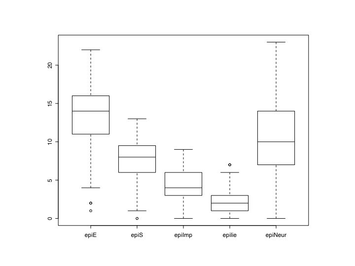
Graphical displays
A quick overview of some of the graphic facilities. See the r.graphics and the plot regressions and how to plot temporal data pages for more details.
For a stunning set of graphics produced with R and the code for drawing them, see addicted to R: R Graph Gallery : Enhance your data visualisation with R.
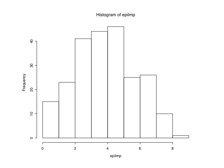
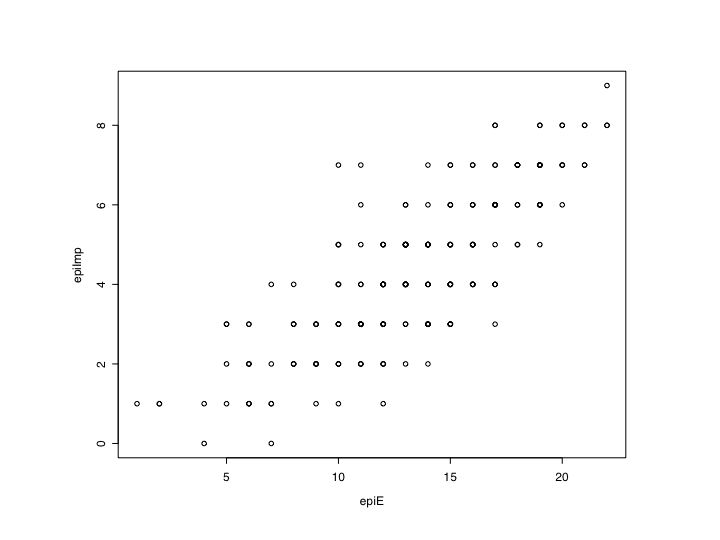
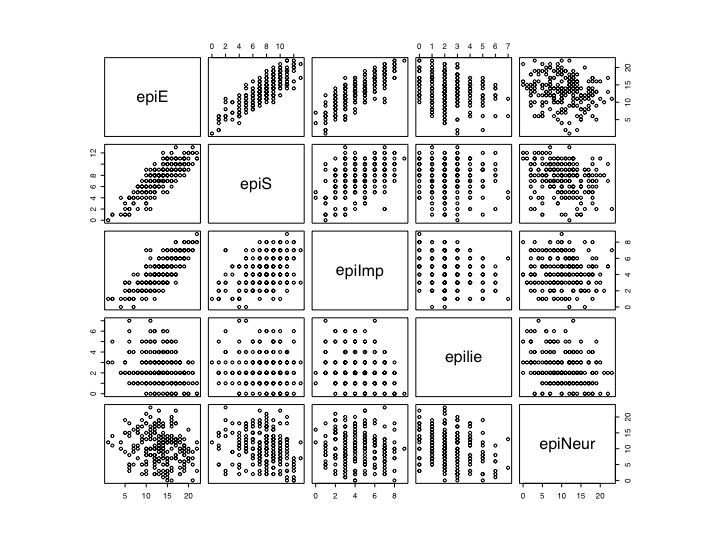
#see the graphic window for the output

boxplot(epi)        #boxplot of the five epi scales
hist(epiE)          #simple histogram
plot(epiE,epiImp)    #simple scatter plot
pairs(epi.df)           #splom plot
boxplot(epi)
hist(epiE)
plot(epiE,epiImp) #Simple scatter plot
pairs(epi) # Basic ScatterPlot Matrix (SPLOM)
More advanced plotting (see r.graphics and r.plotregressions for details)
Inferential Statistics -- Analysis of Variance
The following are examples of Analysis of Variance. A more complete listing and discussion of these examples including the output is in the R.anova page. This section just gives example instructions. See also the ANOVA section of Jonathan Baron's page.
- One Way ANOVA
#tell where the data come from
datafilename="https://personality-project.org/r/datasets/R.appendix1.data"
data.ex1=read.table(datafilename,header=T)   #read the data into a table

aov.ex1 = aov(Alertness~Dosage,data=data.ex1)  #do the analysis of variance
summary(aov.ex1)                                    #show the summary table
print(model.tables(aov.ex1,"means"),digits=3)
	#report the means and the number of subjects/cell
boxplot(Alertness~Dosage,data=data.ex1)
	#graphical summary appears in graphics window
Two Way (between subjects) Analysis of Variance (ANOVA) The standardard 2-way ANOVA just adds another Independent Variable to the model. The example data set is stored at the personality-project.
datafilename="https://personality-project.org/R/datasets/R.appendix2.data"
data.ex2=read.table(datafilename,header=T)   #read the data into a table
data.ex2                                      #show the data
aov.ex2 = aov(Alertness~Gender*Dosage,data=data.ex2)         #do the analysis of variance
summary(aov.ex2)                                    #show the summary table
print(model.tables(aov.ex2,"means"),digits=3)
	#report the means and the number of subjects/cell
boxplot(Alertness~Dosage*Gender,data=data.ex2)
	#graphical summary of means of the 4 cells
attach(data.ex2)
interaction.plot(Dosage,Gender,Alertness)  #another way to graph the means
detach(data.ex2)
One way repeated Measures Repeated measures are some what more complicated. However, Jason French has prepared a very useful tutorial on using R for repeated measures.
                      #Run the analysis:
datafilename="https://personality-project.org/r/datasets/R.appendix3.data"
data.ex3=read.table(datafilename,header=T)   #read the data into a table
data.ex3                                      #show the data
aov.ex3 = aov(Recall~Valence+Error(Subject/Valence),data.ex3)
summary(aov.ex3)
print(model.tables(aov.ex3,"means"),digits=3)
	#report the means and the number of subjects/cell
boxplot(Recall~Valence,data=data.ex3)          #graphical output
Two way repeated measures This gets even more complicated.
datafilename="https://personality-project.org/r/datasets/R.appendix4.data"
data.ex4=read.table(datafilename,header=T)   #read the data into a table
 data.ex4                                      #show the data
 aov.ex4=aov(Recall~(Task*Valence)+Error(Subject/(Task*Valence)),data.ex4 )

summary(aov.ex4)
print(model.tables(aov.ex4,"means"),digits=3)
	#report the means and the number of subjects/cell
boxplot(Recall~Task*Valence,data=data.ex4) #graphical summary of means of the 6 cells
attach(data.ex4)
interaction.plot(Valence,Task,Recall)    #another way to graph the interaction
detach(data.ex4)
- 4 way anova: 2 repeated measures and two between subjects
datafilename="https://personality-project.org/r/datasets/R.appendix5.data"
data.ex5=read.table(datafilename,header=T)   #read the data into a table
#data.ex5                                      #show the data
aov.ex5 =
aov(Recall~(Task*Valence*Gender*Dosage)+Error(Subject/(Task*Valence))+
(Gender*Dosage),data.ex5)

summary(aov.ex5)
print(model.tables(aov.ex5,"means"),digits=3)
	#report the means and the number of subjects/cell
boxplot(Recall~Task*Valence*Gender*Dosage,data=data.ex5)
	#graphical summary of means of the 36 cells
boxplot(Recall~Task*Valence*Dosage,data=data.ex5)
	#graphical summary of means of  18 cells
Reorganizing the data for within subject analyses
The prior examples have assumed one line per unique subject/variable combination. This is not a typical way to enter data. A more typical way (found e.g., in Systat) is to have one row/subject. We need to "stack" the data to go from the standard input to the form preferred by the analysis of variance. Consider the following analyses of 27 subjects doing a memory study of the effect on recall of two presentation rates and two recall intervals. Each subject has two replications per condition. The first 8 columns are the raw data, the last 4 columns collapse across replications. The data are found in a file on the personality project server.
datafilename="/Users/bill/Desktop/R.tutorial/datasets/recall1.data"
recall.data=read.table(datafilename,header=TRUE)
recall.data    #show the data
We can use the "stack() function to arrange the data in the correct manner. We then need to create a new data.frame (recall.df) to attach the correct labels to the correct conditions. This seems more complicated than it really is (although it is fact somewhat tricky). It is useful to list the data after the data frame operation to make sure that we did it correctly. (This and the next two examples are adapted from Baron and Li's page. ) We make use of the rep(), c(), and factor() functions.
rep (operation,number) repeats an operation number times
c(x,y) forms a vector with x and y elements
factor (vector) converts a numeric vector into factors for an ANOVA
More detail on this technique, with comparisons of the original data matrix to the stacked matrix to the data structure version is shown on the r.anova page.
raw=recall.data[,1:8]              #just trial data
#First set some specific paremeters for the analysis -- this allows
numcases=27                  #How many subjects are there?
numvariables=8               #How many repeated measures are there?
numreplications=2            #How many replications/subject?
numlevels1=2                 #specify the number of levels for within subject variable 1
numlevels2=2                 #specify the number of levels for within subject variable 2

stackedraw=stack(raw)        #convert the data array into a vector
                             #add the various coding variables for the conditions
                             #make sure to check that this coding is correct
recall.raw.df=data.frame(recall=stackedraw,
	subj=factor(rep(paste("subj", 1:numcases, sep=""), numvariables)),
	replication=factor(rep(rep(c("1","2"), c(numcases, numcases)),
		numvariables/numreplications)),
	time=factor(rep(rep(c("short", "long"),
		c(numcases*numreplications, numcases*numreplications)),numlevels1)),
	study=rep(c("d45", "d90") ,c(numcases*numlevels1*numreplications,
		numcases*numlevels1*numreplications)))


recall.aov= aov(recall.values ~ time * study + Error(subj/(time * study)), data=recall.raw.df)
	#do the ANOVA
summary(recall.aov)                                #show the output
print(model.tables(recall.aov,"means"),digits=3)   #show the cell means for the anova table
Linear regression
Many statistics used by psychologists and social scientists are special cases of the linear model (e.g., ANOVA is merely the linear model applied to categorical predictors). Generalizations of the linear model include an even wider range of statistical models.
Consider the following models:
- y~x or y~1+x are both examples of simple linear regression with an implicit or explicit intercept.
- y~0+x or y~ -1 +x or y~ x-1 linear regression through the origin
- y ~ A where A is a matrix of categorical factors is a classic ANOVA model.
- y ~ A + x is ANOVA with x as a covariate
- y ~A*B or y~ A + B + A*B ANOVA with interaction terms
- ...
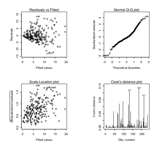
These models can be fitted with the linear model function (lm) and then various summary statistics are available of the fit. The data set is our familiar set of Eysenck Personality Inventory and Big Five Inventory scales with Beck Depression and state and trait anxiety scales as well. The first analysis just regresses BDI on EPI Neuroticism, then we add in Trait Anxiety, and then the N * trait Anx interaction. Note that we need to 0 center the predictors when we have an interaction term if we expect to interpret the additive effects correctly. Centering is done with the scale () function. Graphical summaries of the regession show four plots: residuals as a function of the fitted values, standard errors of the residuals, a plot of the residuals versus a normal distribution, and finally, a plot of the leverage of subjects to determine outliers. Models 5 and 6 predict bdi using the BFI, and model 7 (for too much fitting) looks at the epi and bfi and the interactions of their scales. What follows are the commands for a number of demonstrations. Samples of the commands and the output may be found in the regression page. Further examples show how to find regressions for multiple dependent variables or to find the regression weights from the correlation matrix rather than the raw data.
Produces this outputdatafilename="https://personality-project.org/r/datasets/maps.mixx.epi.bfi.data" #where are the data personality.data =read.file(datafilename) #read the data file colnames(personality.data) #what variables are in the data set? model1 = lm(bdi~epiNeur,data=personality.data) #simple regression of beck depression on Neuroticism summary(model1) # basic statistical summary
Call:
lm(formula = bdi ~ epiNeur, data = personality.data)

Residuals:
     Min       1Q   Median       3Q      Max
-11.9548  -3.1577  -0.7707   2.0452  16.4092

Coefficients:
            Estimate Std. Error t value Pr(>|t|)
(Intercept) -0.32129    0.73070   -0.44    0.661
epiNeur      0.68200    0.06353   10.74   <2e-16 ***
---
Signif. codes:  0 ‘***’ 0.001 ‘**’ 0.01 ‘*’ 0.05 ‘.’ 0.1 ‘ ’ 1

Residual standard error: 4.721 on 229 degrees of freedom
Multiple R-squared:  0.3348,	Adjusted R-squared:  0.3319
F-statistic: 115.3 on 1 and 229 DF,  p-value: < 2.2e-16
To do some graphics
                  #pass parameters to the graphics device
op <- par(mfrow = c(2, 2), # 2 x 2 pictures on one plot
               pty = "s")       # square plotting region,
                                # independent of device size


plot(model1)     #diagnostic plots in the graphics window

model2=lm(bdi~epiNeur+traitanx)    #add in trait anxiety
summary(model2)    #basic output
plot(model2)

anova(model1,model2)             #compare the difference between the two models
model2.5=lm(bdi~epiNeur*traitanx)
	#test for the interaction, note that the main effects are incorrect
summary(model2.5)               #because we need to 0 center the data
anova(model2,model2.5)          #compare the two models

                                #rescale the data to do the analysis
cneur=scale(epiNeur,scale=F)    #0 center epiNeur
zneur=scale(epiNeur,scale=T)     #standardize epiNeur
ctrait = scale(traitanx,scale=F) #0 center traitAnx

model3=lm(bdi~cneur+ctrait+cneur*ctrait)
summary(model3)                    #explicitly list the additive and interactive terms
plot(model3)
model4=lm(bdi~cneur*ctrait)
summary(model4)                    #note how this is exactly the same as the previous model


epi=cbind(epiS,epiImp,epilie,epiNeur)
	#form a new variable "epi" without overall extraversion
epi=as.matrix(epi)      #actually, more useful to treat this variable as a matrix

bfi=as.matrix(cbind(bfext,bfneur,bfagree,bfcon,bfopen))    #create bfi as a matrix as well
epi=scale(epi,scale=T)   #standardize the epi
bfi=scale(bfi,scale=T)   #standardize the bfi

model5=lm(bdi~bfi)                 #model beck depression by the Big 5 inventory
summary(model5)
model6=lm(bdi~bfi+epi)
summary(model6)

model7 = lm(bdi~bfi*epi)
	#additive model of epi and bfi as well as the interactions between the sets
summary(model7)                   #given as an example of overfitting
 ## At end of plotting, reset to previous settings:
     par(op)
Further examples show how multiple regression can be done with multiple dependent variables at the same time and how regressions can be done based upon the correlation matrix rather than the raw data.
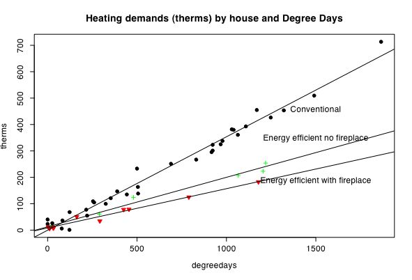
In order to visualize interactions, it is useful to plot regression lines separately for different groups. This is demonstrated in some detail in a real example based upon heating demands of two houses.
Multivariate procedures in R
Scale Construction and Reliability
(This section, written eight years ago, shows how to do the analyses in "vanilla R". I recommend installing the psych package from CRAN and using the more powerful functions in that pacakge.) Follow the various vignettes associated with psych
One of the most common problems in personality research is to combine a set of items into a scale. Questions to ask of these items and the resulting scale are a) what are the item means and variances. b) What are the intercorrelations of the items in the scale. c) What are the correlations of the items with the composite scale. d) what is an estimate of the internal consistency reliability of the scale. (For a somewhat longer discussion of this, see the internal structure of tests.)
The following steps analyze a small subset of the data of a large project (the synthetic aperture personality measurement project at the Personality, Motivation, and Cognition lab). The data represent responses to five items sampled from items measuring extraversion, emotional stability, agreeableness, conscientiousness, and openness taken from the IPIP (International Personality Item Pool) for 200 subjects.
#get the data
datafilename="https://personality-project.org/R/datasets/extraversion.items.txt"
	#where are the data

items=read.table(datafilename,header=TRUE)                    #read the data

attach(items)         #make this the active path
E1=q_262 -q_1480 +q_819 -q_1180 +q_1742  +14
					#find a five item extraversion scale
                    #note that because the item responses ranged from 1-6, to reverse an item
                    #we subtract it from the maximum response possible + the minimum.
                    #Since there were two reversed items, this is the same as adding 14


E1.df = data.frame(q_262 ,q_1480 ,q_819 ,q_1180 ,q_1742 ) #put these items into a data frame

summary(E1.df)                             #give summary statistics for these items
round(cor(E1.df,use="pair"),2)             #correlate the 5 items, rounded off to 2 decimals,
						#use pairwise cases
round(cor(E1.df,E1,use="pair"),2)          #show the item by scale correlations
                                           #define a function to find the alpha coefficient

alpha.scale=function (x,y)   #create a reusable function to find coefficient alpha
	#input to the function are a scale and a data.frame of the items in the scale
        {
                Vi=sum(diag(var(y,na.rm=TRUE)))     #sum of item variance
                Vt=var(x,na.rm=TRUE)                #total test variance
                n=dim(y)[2]     #how many items are in the scale?  (calculated dynamically)
                ((Vt-Vi)/Vt)*(n/(n-1))}             #alpha


E.alpha=alpha.scale(E1,E1.df)
	#find the alpha for the scale E1 made up of the 5 items in E1.df
detach(items)
	#take them out of the search path
Produces the following output:
summary(E1.df)      #give summary statistics for these items
     q_262          q_1480          q_819           q_1180          q_1742
 Min.   :1.00   Min.   :0.000   Min.   :0.000   Min.   :0.000   Min.   :0.000
 1st Qu.:2.00   1st Qu.:2.000   1st Qu.:4.000   1st Qu.:2.000   1st Qu.:3.750
 Median :3.00   Median :3.000   Median :5.000   Median :4.000   Median :5.000
 Mean   :3.07   Mean   :2.885   Mean   :4.565   Mean   :3.295   Mean   :4.385
 3rd Qu.:4.00   3rd Qu.:4.000   3rd Qu.:5.000   3rd Qu.:4.000   3rd Qu.:6.000
 Max.   :6.00   Max.   :6.000   Max.   :6.000   Max.   :6.000   Max.   :6.000


round(cor(E1.df,use="pair"),2)
	#correlate the 5 items, rounded off to 2 decimals, use complete cases
       q_262 q_1480 q_819 q_1180 q_1742
q_262   1.00  -0.26  0.41  -0.51   0.48
q_1480 -0.26   1.00 -0.66   0.52  -0.47
q_819   0.41  -0.66  1.00  -0.41   0.65
q_1180 -0.51   0.52 -0.41   1.00  -0.49
q_1742  0.48  -0.47  0.65  -0.49   1.00


round(cor(E1.df,E1,use="pair"),2)      #show the item by scale correlations
        [,1]
q_262   0.71
q_1480 -0.75
q_819   0.80
q_1180 -0.78
q_1742  0.80

alpha.scale=function (x,y)
	#find coefficient alpha given a scale and a data.frame of the items in the scale
+ 	{
+ 	Vi=sum(diag(var(y,na.rm=TRUE)))     #sum of item variance
+ 	Vt=var(x,na.rm=TRUE)                #total test variance
+   	n=dim(y)[2]                #how many items are in the scale? (calculated dynamically)
+   	((Vt-Vi)/Vt)*(n/(n-1))}    #alpha
>
>
>

E.alpha=alpha.scale(E1,E1.df,5)
	#find the alpha for the scale E1 made up of the 5 items in E1.df

E.alpha
[1] 0.822683
Using the alpha function from psych
Alternatively, this same analysis could have been done using the alpha function from the psych package:
E1.df <- with(items,data.frame(q_262 ,q_1480 ,q_819 ,q_1180 ,q_1742 ))
	#another way to create the data.frame
alpha(E1.df)


Reliability analysis
Call: alpha(x = E1.df)

  raw_alpha std.alpha G6(smc) average_r mean   sd
      0.82      0.83    0.83      0.49  3.6 0.52

 Reliability if an item is dropped:
        raw_alpha std.alpha G6(smc) average_r
q_262        0.82      0.82    0.80      0.53
q_1480-      0.79      0.80    0.76      0.49
q_819        0.77      0.77    0.74      0.46
q_1180-      0.79      0.79    0.77      0.49
q_1742       0.77      0.78    0.77      0.46

 Item statistics
          n    r r.cor r.drop mean  sd
q_262   200 0.70  0.58   0.52  3.1 1.5
q_1480- 200 0.76  0.70   0.60  2.9 1.4
q_819   200 0.82  0.78   0.69  4.6 1.2
q_1180- 200 0.77  0.69   0.62  3.3 1.5
q_1742  200 0.80  0.74   0.67  4.4 1.4

Non missing response frequency for each item
          0    1    2    3    4    5    6 miss
q_262  0.00 0.18 0.20 0.22 0.22 0.12 0.06    0
q_1480 0.00 0.18 0.25 0.18 0.26 0.08 0.03    0
q_819  0.00 0.02 0.06 0.12 0.17 0.42 0.22    0
q_1180 0.01 0.14 0.19 0.16 0.30 0.14 0.06    0
q_1742 0.00 0.04 0.08 0.13 0.22 0.26 0.27    0
Warning message:
In alpha(E1.df) :
  Some items were negatively correlated with total scale and were automatically reversed
Scoring multiple choice tests
If you are using multiple choice tests and want to score the items following a key, it is possible to use the power of R for data manipulation:
Consider the problem of scoring a multiple choice test where we are interested in the number of items correct for each person. Define a scoring key vector and then score as 1 each item match with that key. Then find the number of 1s for each subject. We use the Iris data set as an example.
iris2 <- round(iris[1:10,1:4])   #get a sample data set
key <- iris2[1,]    #make up an arbitary answer key
score <- t(t( rowSums((iris2 == c(key[]))+0)))   #look for correct item and add them up
mydata <- data.frame(iris2,score)     #
key         #what is the scoring key
mydata      #show the data with the number of items that match the key
(Thanks to Gabor Grothendieck and R help for this trick.) A more typical example using the score.multiple.choice function can be done on the iqitems example in psych
data(iqitems)
iq.keys <- c(4,4,3,1,4,3,2,3,1,4,1,3,4,3)
score.multiple.choice(iq.keys,iqitems)
#convert them to true false
iq.scrub <- scrub(iqitems,isvalue=0)  #first get rid of the zero responses
iq.tf <-  score.multiple.choice(iq.keys,iq.scrub,score=FALSE)
#convert to wrong (0) and correct (1) for analysis
describe(iq.tf)

Call: score.multiple.choice(key = iq.keys, data = iqitems)

(Unstandardized) Alpha:
[1] 0.63

Average item correlation:
[1] 0.11

item statistics
     key    0    1    2    3    4    5    6 miss    r    n mean   sd  skew kurtosis   se
iq1    4 0.04 0.01 0.03 0.09 0.80 0.02 0.01    0 0.59 1000 0.80 0.40 -1.51     0.27 0.01
iq8    4 0.03 0.10 0.01 0.02 0.80 0.01 0.04    0 0.39 1000 0.80 0.40 -1.49     0.22 0.01
iq10   3 0.10 0.22 0.09 0.37 0.04 0.13 0.04    0 0.35 1000 0.37 0.48  0.53    -1.72 0.02
iq15   1 0.03 0.65 0.16 0.15 0.00 0.00 0.00    0 0.35 1000 0.65 0.48 -0.63    -1.60 0.02
iq20   4 0.03 0.02 0.03 0.03 0.85 0.02 0.01    0 0.42 1000 0.85 0.35 -2.00     2.01 0.01
iq44   3 0.03 0.10 0.06 0.64 0.02 0.14 0.01    0 0.42 1000 0.64 0.48 -0.61    -1.64 0.02
iq47   2 0.04 0.08 0.59 0.06 0.11 0.07 0.05    0 0.51 1000 0.59 0.49 -0.35    -1.88 0.02
iq2    3 0.07 0.08 0.31 0.32 0.15 0.05 0.02    0 0.26 1000 0.32 0.46  0.80    -1.37 0.01
iq11   1 0.04 0.87 0.03 0.01 0.01 0.01 0.04    0 0.54 1000 0.87 0.34 -2.15     2.61 0.01
iq16   4 0.05 0.05 0.08 0.07 0.74 0.01 0.00    0 0.56 1000 0.74 0.44 -1.11    -0.77 0.01
iq32   1 0.04 0.54 0.02 0.14 0.10 0.04 0.12    0 0.50 1000 0.54 0.50 -0.17    -1.97 0.02
iq37   3 0.07 0.10 0.09 0.26 0.13 0.02 0.34    0 0.23 1000 0.26 0.44  1.12    -0.74 0.01
iq43   4 0.04 0.07 0.04 0.02 0.78 0.03 0.00    0 0.50 1000 0.78 0.41 -1.35    -0.18 0.01
iq49   3 0.06 0.27 0.09 0.32 0.14 0.08 0.05    0 0.28 1000 0.32 0.47  0.79    -1.38 0.01
> #convert them to true false
> iq.scrub <- scrub(iqitems,isvalue=0)  #first get rid of the zero responses
> iq.tf <-  score.multiple.choice(iq.keys,iq.scrub,score=FALSE)
#convert to wrong (0) and correct (1) for analysis
> describe(iq.tf)
     var   n mean   sd median trimmed mad min max range  skew kurtosis   se
iq1    1 965 0.83 0.38      1    0.91   0   0   1     1 -1.75     1.08 0.01
iq8    2 972 0.82 0.38      1    0.90   0   0   1     1 -1.68     0.83 0.01
iq10   3 900 0.41 0.49      0    0.39   0   0   1     1  0.36    -1.88 0.02
iq15   4 968 0.67 0.47      1    0.72   0   0   1     1 -0.73    -1.46 0.02
iq20   5 972 0.88 0.33      1    0.97   0   0   1     1 -2.31     3.36 0.01
iq44   6 971 0.66 0.47      1    0.71   0   0   1     1 -0.69    -1.52 0.02
iq47   7 955 0.61 0.49      1    0.64   0   0   1     1 -0.47    -1.78 0.02
iq2    8 929 0.34 0.47      0    0.30   0   0   1     1  0.68    -1.54 0.02
iq11   9 964 0.90 0.30      1    1.00   0   0   1     1 -2.63     4.93 0.01
iq16  10 953 0.78 0.41      1    0.85   0   0   1     1 -1.35    -0.19 0.01
iq32  11 962 0.56 0.50      1    0.58   0   0   1     1 -0.26    -1.93 0.02
iq37  12 928 0.27 0.45      0    0.22   0   0   1     1  1.01    -0.99 0.01
iq43  13 958 0.81 0.39      1    0.89   0   0   1     1 -1.61     0.60 0.01
iq49  14 939 0.34 0.47      0    0.30   0   0   1     1  0.69    -1.53 0.02
Factor Analysis
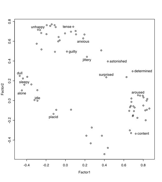
Core R includes a maximum likelihood factor analysis function (factanal) and the psych package includes five alternative factor extraction options within one function, fa. For the following analyses, we will use data from the Motivational State Questionnaire (MSQ) collected in several studies. This is a subset of a larger data set (with N>3000 that has been analyzed for the structure of mood states (Rafaeli, Eshkol and Revelle, William (2006), A premature consensus: Are happiness and sadness truly opposite affects? Motivation and Emotion, 30, 1, 1-12.). The data set includes EPI and BFI scale scores (see previous examples).
#specify the name and address of the remote file
datafilename="https://personality-project.org/r/datasets/maps.mixx.msq1.epi.bf.txt"
#note that it is also available as built in example in the psych package named msq
msq =read.table(datafilename,header=TRUE)  #read the data file
mymsq=msq[,2:72]             #select the subset of items in the MSQ

mymsq[mymsq=="9"] = NA       # change all occurences of 9 to be missing values
mymsq <- data.frame(mymsq)    #convert the input matrix into a data frame for easier manipulation

names(mymsq)                        #what are the variables?
describe(mymsq)                     #basic summary statistics -- check for miscodings

cleaned <- na.omit(mymsq)     #remove the cases with missing values
f2 <- fa(cleaned,2,rotation="varimax")   		#factor analyze the resulting item
#(f2)                                              #show the result
load=loadings(f2)
print(load,sort=TRUE,digits=2,cutoff=0.01)  #show the loadings
plot(load)                                 #plot factor 1 by 2
identify(load,labels=names(msq))
 	#put names of selected points onto the figure  -- to stop, click with command key
 plot(f2,labels=names(msq))
It is also possible to find and save the covariance matrix from the raw data and then do subsequent analyses on this matrix. This clearly saves computational time for large data sets. This matrix can be saved and then reloaded.
 msqcovar=cov(mymsq,use="pair")  #find the covariance matrix for later factoring
 f3=factanal(x, factors=3, data = NULL, covmat = msqcovar, n.obs = 300,start=NULL,
 	rotation = "varimax")
 f4=factanal(x, factors=4, data = NULL, covmat = msqcovar, n.obs = 300,start=NULL,
 	rotation = "varimax")
The fa function will do maximimum likelihood but defaults to do a minimum residual (min-res) solution with an oblimin rotation. The similarity of the three different solutions may be found by using the factor.congruence function.
factor.congruence(list(f2,f3,f4))


          MR1   MR2 Factor1 Factor2 Factor3 Factor1 Factor2 Factor3 Factor4
MR1      1.00 -0.01    0.99   -0.09   -0.14    0.99   -0.09   -0.02   -0.64
MR2     -0.01  1.00   -0.11    0.99   -0.25   -0.08    0.99   -0.37    0.18
Factor1  0.99 -0.11    1.00   -0.18   -0.07    0.99   -0.18    0.06   -0.64
Factor2 -0.09  0.99   -0.18    1.00   -0.14   -0.15    1.00   -0.27    0.29
Factor3 -0.14 -0.25   -0.07   -0.14    1.00   -0.03   -0.13    0.95    0.46
Factor1  0.99 -0.08    0.99   -0.15   -0.03    1.00   -0.15    0.06   -0.56
Factor2 -0.09  0.99   -0.18    1.00   -0.13   -0.15    1.00   -0.25    0.25
Factor3 -0.02 -0.37    0.06   -0.27    0.95    0.06   -0.25    1.00    0.19
Factor4 -0.64  0.18   -0.64    0.29    0.46   -0.56    0.25    0.19    1.00
Very Simple Structure
There are multiple ways to determine the appropriate number of factors in exploratory factor analysis. Routines for the Very Simple Structure (VSS) criterion allow one to compare solutions of varying complexity and for different number of factors. Alternatives include the scree test. To use these routines on a data set with items, myitems,:
library(psych)
my.vss <- VSS(mydata,n=8,rotate="none",diagonal=FALSE,...)   #compares up to 8 factors
op <- par(mfrow=c(1,2))  #make a two panel graph
VSS.plot(my.vss)  #shows a simple summary of VSS
VSS.scree(cor(mydata),main="scree plot of principal components of mydata")
Omega: General Factor Saturation of a test
McDonald has proposed coefficient omega as an estimate of the general factor saturation of a test. Revelle and Zinbarg (2009) discuss multiple estimates of reliability, Zinbarg, Revelle, Yovel and Li (2005) compare McDonald's Omega to Chronbach's alpha and Revelle's beta. They conclude that omega is the best estimate. (See also Zinbarg et al., 2006)
One way to find omega is to do a factor analysis of the original data set, rotate the factors obliquely, do a Schmid Leiman transformation, and then find omega. Here we present code to do that. This code is included in the psych package of routines for personality research that may be loaded from the CRAN repository or, for the the recent development version, from the local repository at https://personality-project.org/r.
Beta: General Factor Saturation of a test
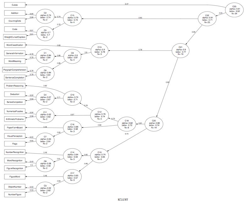
Beta, an alternative to omega, is defined as the worst split half reliability. It can be estimated by using ICLUST (Revelle, 1979), a hierarchical clustering algorithm originally developed for main frames and written in Fortran and that is now part of the psych package. (For a very complimentary review of why the ICLUST algorithm is useful in scale construction, see Cooksey and Soutar, 2005). What took multiple years and about 2500 lines of code in Fortrantook about 4 days and 100 lines of R.
Factor rotations
Rotations available in the basic R installation are Varimax and Promax. A powerful additional set of oblique transformations including Oblimin, Oblimax, etc. are available in the GPArotations package from Cran. Using this package, it is also possible to do a Schmid Leiman transformation of a hierarchical factor structure to estimate the general factor loadings and general factor saturation of a test. (see omega .)
Cluster Analysis
A common data reduction technique is to cluster cases (subjects). Less common, but particularly useful in psychological research, is to cluster items (variables). This may be thought of as an alternative to factor analysis, based upon a much simpler model. The cluster model is that the correlations between variables reflect that each item loads on at most one cluster, and that items that load on those clusters correlate as a function of their respective loadings on that cluster and items that define different clusters correlate as a function of their respective cluster loadings and the intercluster correlations. Essentially, the cluster model is a factor model of complexity one (see VSS).
An example of clustering variables can be seen using the ICLUST algorithm to the 24 tests of mental ability of Harman and then using the Graphviz program to show the results.
r.mat<- Harman74.cor$cov
ic.demo <- ICLUST(r.mat)
ICLUST.graph(ic.demo,out.file = ic.demo.dot)
Multidimensional scaling
Given a set of distances (dis-similarities) between objects, is it possible to recreate a dimensional representation of those objects?
Model: Distance = square root of sum of squared distances on k dimensions dxy = √∑(xi-yi)2
Data: a matrix of distances
Find the dimensional values in k = 1, 2, ... dimensions for the objects that best reproduces the original data.
Example: Consider the distances between nine American cities. Can we represent these cities in a two dimensional space.
See the pages on multidimensional scaling and Thurstonian scaling.
Jan de Leeuw at UCLA is converting a number of mds packages including the ALSCAL program for R. See his page at https://www.cuddyvalley.org/psychoR/code. ALSCAL generalizes the INDSCAL algorithm for individual differences in multiple dimensional scaling.
Further topics
Structural Equation Modeling
Structural equation models combine measurement models (e.g., reliability) with structural models (e.g., regression). The sem package, developed by John Fox, the lavaan package by Yves Rosseel, and the OpenMx package by Steve Bolker allow for most structural equation models. To use then, add the sem, lavaan or OpenMx packages.
Structural Equation Modeling may be thought of as regression corrected for attentuation. The sem package developed by John Fox uses the RAM path notation of Jack McCardle and is fairly straightforward. Fox has prepared a brief description of SEM techniques as an appendix to his statistics text. The examples in the package are quite straightforward. A text book, such as John Loehlin's Latent Variable Models (4th Edition) is helpful in understanding the algorithm.
Demonstrations of using the sem package for several of the Loehlin problems are discussed in more detail on a separate page. In addition, lecture notes for a course on sem (primarily using R) are available at the syllabus for my sem course.
Multilevel Models/ Hierarchical Level Models
HLM can be done using the lme package. See the discussion in the R newsletter, Vol 3/3 by Lockwood, Doran, and McCaffrey. Also see the relevant pdf appendix of John Fox's text on applied regression.
Item Response Theory using R
Item Response Theory is a model that considers individual differences in ability as well as item difficulty. It is sometimes called the "new" psychometrics (as contrasted to "classic" psychometrics of traditional test theory.) Essentially, classic psychometrics estimates person scores by assuming items are random replicates of each other. Precision of measurement is expressed in terms of the reliability which is the ratio of "true" score variance to total test variance. Reliability is thus a between person concept. IRT estimates person scores as well as item difficulty (endorsement) scores. Precision of measurement may be estimated in terms of the patterns of scores of a single individual and does not require between person variability. Although the "new" and "classic" psychometrics give very similar estimates of person scores, the ability to do tailored tests and to consider the metric properties of the scales makes IRT very useful. IRT models differ in their complexity. The one parameter model assumes items all have equal discriminability and differ only in their difficulty. The two parameter model assumes items differ in difficulty and discriminability, the three parameter model assumes items differ in the ease of guessing. Although developed for binary items (correct versus incorrect), generalizations of IRT to multiresponse formats are very useful.
For a detailed demonstration of how to do 1 parameter IRT (the Rasch Model) see Jonathan Baron and Yuelin Li's tutorial on R. A more useful package for latent trait modeling (e.g., Rasch modeling and item response theory) (ltm) has now been released by Dimitris Rizopoulos. Note that to use this package, you must first install the MASS, gtools, and msm packages.
The ltm package allows for 1 parameter (Rasch) and two parameter (location and discrimination) modeling of a single latent trait assessed by binary items varying in location and discrimination. Procedures include graphing the results as well as anova comparisons of nested models.
The 2 parameter IRT model is essentially a reparameterization of the factor analytic model and thus can be done through factor analysis. This is done in the irt.fa and score.irt functions in psych.
Simulating data structures and probability tables
There are at least 20 distributions available including the normal, the binomial, the exponential, the logistic, Poisson, etc. Each of these can be accessed for density ('d'), cumulative density ('p'), quantile ('q') or simulation ('r' for random deviates). Thus, to find out the probability of a normal score of value x from a distribution with mean=m and sd = s,
pnorm(x,mean=m, sd=s), eg.
pnorm(1,mean=0,sd=1)
[1] 0.8413447
which is the same as
pnorm(1)       #default values of mean=0, sd=1 are used)
pnorm(1,1,10)  #parameters may be passed if in default order or by name
Examples of using R to demonstrate the central limit theorem or to produce circumplex structure of personality items are useful ways to teach sampling theory or to explore artifacts in measurement.
Simulating a simple correlation between two variables based upon their correlation with a latent variable:
samplesize=1000
size.r=.6
theta=rnorm(samplesize,0,1)      #generate some random normal deviates
e1=rnorm(samplesize,0,1)         #generate errors for x
e2=rnorm(samplesize,0,1)         #generate errors for y
weight=sqrt(size.r)              #weight as a function of correlation
x=weight*theta+e1*sqrt(1-size.r) #combine true score (theta) with error
y=weight*theta+e2*sqrt(1-size.r)
cor(x,y)                          #correlate the resulting pair
df=data.frame(cbind(theta,e1,e2,x,y))  #form a data frame to hold all of the elements
round(cor(df),2)               #show the correlational structure
pairs.panels(df)                #plot the correlational structure (assumes psych package)
The use of the mvtnorm package and the rmvnorm(n, mean, sigma) function allows for creating random covariance matrices with a specific structure.
e.g., using the sample sizes and rs from above:
library(mvtnorm)
samplesize=1000
size.r=.6
sigmamatrix <- matrix( c(1,sqrt(size.r),sqrt(size.r),sqrt(size.r),1,size.r,
	sqrt(size.r),size.r,1),ncol=3)
xy <- rmvnorm(samplesize,sigma=sigmamatrix)
round(cor(xy),2)
pairs.panels(xy) 	#assumes the psych package
Another simulation shows how to create a multivariate structure with a particular measurement model and a particular structural model. This example produces data suitable for demonstrations of regression, correlation, factor analysis, or structural equation modeling.
The particular example assumes that there are 3 measures of ability (GREV, GREQ, GREA), two measures of motivation (achievment motivation and anxiety), and three measures of performance (Prelims, GPA, MA). These titles are, of course, arbitrary and can be changed easily. These (simulated) data are used in various lectures of mine on Factor Analysis and Psychometric Theory. Other examples of simulation of item factor structure include creating circumplex structured correlation matrices.
Simulations may also be used to teach concepts in experimental design and analysis. Several simulations of the additive and interactive effects of personality traits with situational manipulations of mood and arousal compare alternative ways of analyzing data.
Finally, a simple simulation to generate and test circumplex versus structures in two dimensions has been added.
Adding new commands (functions) packages or libraries
A very powerful feature of R is that it is extensible. That is, one can write one's own functions to do calculations of particular interest. These functions can be saved as external file that can be accessed using the source command. For example, I frequently use a set of routines that find the alpha reliability of a set of scales, or to draw scatter plots with histograms on the diagonal and font sizes scaled to the absolute value of the correlation. Another set of routines applies the Very Simple Structure (VSS) criterion for determining the optimal number of factors. I originally stored these two sets of files (vss.r and useful.r) and then added them into my programs by using the source command.
source("https://personality-project.org/r/useful.r")  #some basic data manipulation procedures
source("https://personality-project.org/r/vss.r")     #the Very Simple Structure package
However, an even more powerful option is to create packages of frequently used code. These packages can be stored on local "repositories" if they appeal to members of small work groups, or can be added to the CRAN master repository. Guidelines for creating packages are found in the basic help menus. Notes on how to create a specific package (i.e., the psych package) and install it as a repository are meant primarily for Mac users. More extensive discussions for PCs have also been developed.
The package "psych" was added to CRAN in about 2005 and is now (September, 2020) up to version 2.0.9. (I changed the numbering system to reflect year and month of release as I passed the 100th release). As I find an analysis that I need to do that is not easily done using the standard packages, I supplement the psych package. I encourage the reader to try it. The manual is available on line or as part of the package.
To add a package from CRAN (e.g, sem, GPArotation, psych), go to the R package installer, and select install. Then, using the R package Manager, load that package.
Although it is possible to add the psych package from the personality-project.org web page, it is a better idea to use CRAN. You can select the other repository option in the R Package Installer and set it to https://personality-project.org/r . A list of available packages stored there will be displayed. Choose the one you want and then load it with the R package manager. Currently, there is only one package (psych) there. This version will be the current development version will be at least as new as what is on the CRAN site. You must specify that you want a source file if use the personality-project.org/r repository. As of now (May, 2014), the psych package contains more than a 360 functions including the following ones:
| psych-package | A package for personality, psychometric, and psychological research |
| %+% | A function to add two vectors or matrices |
| alpha.scale | Cronbach alpha for a scale |
| circ.sim | Generate simulated data structures for circumplex or simple structure |
| circ.simulation | Simulations of circumplex and simple structure |
| circ.tests | Apply four tests of circumplex versus simple structure |
| cluster.cor | Find correlations of composite variables from a larger matrix |
| cluster.fit | cluster Fit: fit of the cluster model to a correlation matrix |
| cluster.loadings | Find item by cluster correlations, corrected for overlap and reliability |
| correct.cor | Find dis-attenuated correlations and give alpha reliabilities |
| count.pairwise | Count number of pairwise cases for a data set with missing (NA) data. |
| describe | Basic descriptive statistics useful for psychometrics |
| describe.by | Basic summary statistics by group |
| eigen.loadings | Extract eigen vectors, eigen values, show loadings |
| error.crosses | Plot x and y error bars |
| factor.congruence | Coefficient of factor congruence |
| factor.fit | How well does the factor model fit a correlation matrix. Part of the VSS package |
| factor.model | Find R = F F' + U2 is the basic factor model |
| fa | Minimum Residual, Principal Axis, GLS, MLE factor analysis |
| factor.pa | Principal Axis Factor Analysis |
| factor.residuals | R* = R- F F' |
| factor.rotate | "Hand" rotate a factor loading matrix |
| factor2cluster | Extract cluster definitions from factor loadings |
| fisherz | Fisher z transform of r |
| geometric.mean | Find the geometric mean of a vector or columns of a data.frame. |
| harmonic.mean | Find the harmonic mean of a vector, matrix, or columns of a data.frame |
| ICLUST | ICLUST: Item Cluster Analysis - Hierarchical cluster analysis using psychometric principles |
| ICLUST | iclust: Item Cluster Analysis - Hierarchical cluster analysis using psychometric principles |
| ICLUST.cluster | Function to form hierarchical cluster analysis of items |
| ICLUST.graph | create control code for ICLUST graphical output |
| ICLUST.sort | sort items by absolute size of cluster loadins |
| irt.fa | Item Response Theory using factor analysis of tetrachoric or polychoric correlations |
| irt.0p | Item Response Theory estimate of theta (ability) using a Rasch (like) model |
| irt.1p | Item Response Theory estimate of theta (ability) using a Rasch (like) model |
| irt.2p | Item Response Theory estimate of theta (ability) using a Rasch (like) model |
| irt.discrim | Simple function to estimate item difficulties using IRT concepts |
| irt.item.diff.rasch | Simple function to estimate item difficulties using IRT concepts |
| irt.person.rasch | Item Response Theory estimate of theta (ability) using a Rasch (like) model |
| kurtosi | Kurtosis of a vector, matrix, or data frame |
| make.hierarchical | Create a population or sample correlation matrix with hierachical structure. |
| mat.regress | Multiple Regression from matrix input |
| multi.hist | Multiple histograms on one screen |
| omega | Calculate the omega estimate of factor saturation |
| paired.r | Test the difference between paired correlations |
| pairs.panels | SPLOM, histograms and correlations for a data matrix |
| panel.cor | SPLOM, histograms and correlations for a data matrix |
| panel.hist | SPLOM, histograms and correlations for a data matrix |
| phi | Find the phi coefficient of correlation between two dichotomous variables |
| phi2poly | Convert a phi coefficient to a polychoric correlation |
| polychoric | Find polychoric correlations |
| principal | Principal components analysis |
| psych | A package for personality, psychometric, and psychological research |
| psycho.demo | Create demo data for psychometrics |
| read.clipboard | shortcut for reading from the clipboard |
| schmid | Apply the Schmid Leiman transformation to a correlation matrix |
| score.alpha | Score scales and find Cronbach's alpha as well as associated statistics |
| score.items | Score item composite scales and find Cronbach's alpha as well as associated statistics |
| skew | Calculate skew for a vector, matrix, or data.frame |
| VSS | Apply the Very Simple Structure criterion to determine the appropriate number of factors. |
| VSS.parallel | Compare real and random VSS solutions |
| VSS.plot | Plot VSS fits |
| VSS.scree | Plot a scree test |
| VSS.simulate | create VSS like data |
To install the psych package using a Mac, go to the Package Installer Menu option, choose binary, and then psych and it should get the package. To get the most recent release of psych, you can go the personality-project.org repository. (Use other repository in the download packages menu.) Uncheck the "binary" option. This is a source file.
To install on a PC, just use the version on CRAN. Use the package installer option and choose psych.
Once installed, the package can be activated by using the package manager (or just issuing the package(psych) command.
A (partial) list of useful commands
See A short summary of useful R commands for more detail. In addition, the Rpad.pdf reference card file is a very important aid to remembering the many commands available.
Input and display
                                         #read files with labels in first row
read.table(filename,header=TRUE)           #read a tab or space delimited file
read.table(filename,header=TRUE,sep=',')   #read csv files (comma separated)

x=c(1,2,4,8,16 )                             #create a data vector with specified elements
y=c(1:8,1:4)                               #creat a data vector with 12 entries
matr=rbind(1:8,1:4)                         #create two rows in a    2 * 8 matrix
matc=cbind(1:8,1:4)                         #create two columns in a 8 * 2 matrix
n=10
x1=c(rnorm(n))                              #create a n item vector of random normal deviates
y1=c(runif(n))+n
	#create another n item vector that has n added to each random uniform distribution
z=rbinom(n,size,prob)
	#create n samples of size "size" with probability prob from the binomialitem
sample(x, size, replace = FALSE, prob = NULL)
	#take a sample (with or without replacement) of size from x

vect=c(x,y)                                #combine them into one vector of length 2n
mat=cbind(x,y)                             #combine them into a n x 2 matrix (column wise)
mat[4,2]                                   #display the 4th row and the 2nd column
mat[3,]                                    #display the 3rd row
mat[,2]                                    #display the 2nd column
mat=cbind(rep(1:4,2),rep(4:1,2))           #create a 8 * 2 matrix with repeating elements
subset(data,logical)                       #those objects meeting a logical criterion
subset(data.df,select=variables,logical)
	#get those objects from a data frame that meet a criterion
moving around
ls()                                 #list the variables in the workspace
rm(x)                                #remove x from the workspace
rm(list=ls())                        #remove all the variables from the workspace
attach(mat)                          #make the names of the variables in the matrix available
detach(mat)                          #releases the names
new=old[,-n]                         #drop the nth column
new=old[n,]                          #drop the nth row
new=subset(old,logical)              #select those cases that meet the logical condition
complete = subset(data,complete.cases(data))
	#find those cases with no missing values
new=old[n1:n2,n3:n4]              #select the n1 through n2 rows of variables n3 through n4)
data manipulation
x.df=data.frame(x1,x2,x3 ...)        #combine different kinds of data into a data frame
	as.data.frame()
	is.data.frame()
x=as.matrix()
scale()         #converts a data frame to standardized scores
factor() 	#converts a numeric variable into a factor (essential for ANOVA)
gl(n,k,length)	#makes an n-level,k replicates, length long vectof factors
y <- edit(x) 	#opens a screen editor and saves changes made to x intoy
fix(x)		#opens a screen editor window and makes and saves changes to x
Statistics and transformations
 max()
 min()
 mean()
 median()
 sum()
 var()     		#produces the variance covariance matrix
 sd()      		#standard deviation
 mad()     		#(median absolute deviation)
 fivenum() 		#Tukey fivenumbers min, lowerhinge, median, upper hinge, max
 scale(data,scale=T)   	#centers around the mean and scales by the sd)
 colSums(), rowSums(), colMeans(), rowMeans()   #see also apply(x,1,sum)
 rowsum(x,group)     	#sum by group

 cor(x,y,use="pair")
 	#correlation matrix for pairwise complete data, use="complete" for complete cases

 t.test(x,y) #x is a data vector, y is a grouping vector  independent groups
 t.test(x,y,pair=TRUE) #x is a data vector, y is a grouping vector --  paired groups
 pairwise.t.test(x,g) does multiple comparisons of all groups defined by g

 aov(x~y,data=datafile)  #where x and y can be matrices
	 aov.ex1 = aov(Alertness~Dosage,data=data.ex1)
	 	#do the analysis of variance or
	 aov.ex2 = aov(Alertness~Gender*Dosage,data=data.ex2)
	 	#do a two way analysis of variance
	summary(aov.ex1)
		#show the summary table
	print(model.tables(aov.ex1,"means"),digits=3)
		#report the means and the number of subjects/cell
	boxplot(Alertness~Dosage,data=data.ex1)
		#graphical summary appears in graphics window

 lm(x~y,data=dataset)                      #basic linear model where x and y can be matrices

 lm(Y~X)                                 #Y and X can be matrices
 lm(Y~X1+X2)
 lm(Y~X|W)                               #separate analyses for each level of W
 solve(A,B)                              #inverse of A * B   - used for linear regression
 solve(A)                                #inverse of A
Useful additional commands
     colSums (x, na.rm = FALSE, dims = 1)
     rowSums (x, na.rm = FALSE, dims = 1)
     colMeans(x, na.rm = FALSE, dims = 1)
     rowMeans(x, na.rm = FALSE, dims = 1)
     rowsum(x, group, reorder = TRUE, ...)
     	#finds row sums for each level of a grouping variable
     apply(X, MARGIN, FUN, ...)
     	#applies the function (FUN) to either rows (1) or columns (2) on object X
     apply(x,1,min)
    	#finds the minimum for each row
     apply(x,2,max)
     	#finds the maximum for each column
     col.max(x)
     	#another way to find which column has the maximum value for each row
     which.min(x)
     which.max(x)
     z=apply(big5r,1,which.min)
     	#tells the row with the minimum value for every column
Graphics
stem()                                   #stem and leaf diagram

par(mfrow=c(2,1))                        #number of rows and columns to graph

boxplot(x,notch=T,names= grouping, main="title")                  #boxplot (box and whiskers)

hist()                                   #histogram
plot()
  plot(x,y,xlim=range(-1,1),ylim=range(-1,1),main=title)
  par(mfrow=c(1,1))     #change the graph window back to one figure
  symb=c(19,25,3,23)
  colors=c("black","red","green","blue")
  charact=c("S","T","N","H")
  plot(x,y,pch=symb[group],col=colors[group],bg=colors[condit],cex=1.5,main="main title")
  points(mPA,mNA,pch=symb[condit],cex=4.5,col=colors[condit],bg=colors[condit])

curve()
  abline(a,b)
  abline(a, b, untf = FALSE, ...)
  abline(h=, untf = FALSE, ...)
  abline(v=, untf = FALSE, ...)
  abline(coef=, untf = FALSE, ...)
  abline(reg=, untf = FALSE, ...)

identify()
	plot(eatar,eanta,xlim=range(-1,1),ylim=range(-1,1),main=title)
	identify(eatar,eanta,labels=labels(energysR[,1])  )
		#dynamically puts names on the plots
locate()
pairs()                                  #SPLOM (scatter plot Matrix)

matplot ()                             #ordinate is row of the matrix
biplot ()                              #factor loadings and factor scores on same graph
coplot(x~y|z)                          #x by y conditioned on z
symb=c(19,25,3,23)                              #choose some nice plotting symbols
colors=c("black","red","green","blue")          #choose some nice colors

barplot()                  #simple bar plot
interaction.plot ()         #shows means for an ANOVA design

plot(degreedays,therms)               #show  the data points
by(heating,Location,function(x) abline(lm(therms~degreedays,data=x)))
	#show the best fitting regression for each group


x= recordPlot()            #save the current plot device output in the object x
replayPlot(x)              #replot object x
dev.control                #various control functions for printing/saving graphic files
same aspnorm(1,mean=0,sd=1) [1] 0.8413447
pnorm(1)       #default values of mean=0, sd=1 are used)
pnorm(1,1,10)  #parameters may be passed if in default order or by name
Examples of using R to demonstrate the central limit theorem or to produce circumplex structure of personality items are useful ways to teach sampling theory or to explore artifacts in measurement.
Simulating a simple correlation between two variables based upon their correlation with a latent variable:
samplesize=1000
size.r=.6
theta=rnorm(samplesize,0,1)      #generate some random normal deviates
e1=rnorm(samplesize,0,1)         #generate errors for x
e2=rnorm(samplesize,0,1)         #generate errors for y
weight=sqrt(size.r)              #weight as a function of correlation
x=weight*theta+e1*sqrt(1-size.r) #combine true score (theta) with error
y=weight*theta+e2*sqrt(1-size.r)
cor(x,y)                          #correlate the resulting pair
df=data.frame(cbind(theta,e1,e2,x,y))  #form a data frame to hold all of the elements
round(cor(df),2)               #show the correlational structure
pairs.panels(df)                #plot the correlational structure (assumes psych package)
The use of the mvtnorm package and the rmvnorm(n, mean, sigma) function allows for creating random covariance matrices with a specific structure.
e.g., using the sample sizes and rs from above:
library(mvtnorm)
samplesize=1000
size.r=.6
sigmamatrix <- matrix( c(1,sqrt(size.r),sqrt(size.r),sqrt(size.r),1,size.r,
	sqrt(size.r),size.r,1),ncol=3)
xy <- rmvnorm(samplesize,sigma=sigmamatrix)
round(cor(xy),2)
pairs.panels(xy) 	#assumes the psych package